3D Markerless Pose Estimation with DeepLabCut: A Complete Guide for Biomedical Researchers
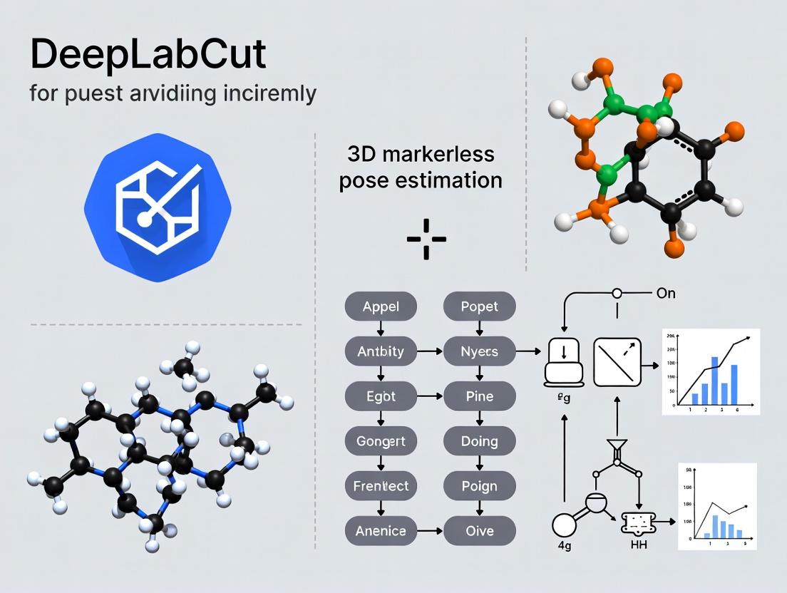
This comprehensive guide explores DeepLabCut (DLC) for 3D markerless pose estimation, a transformative tool for quantifying animal and human behavior in biomedical research.
3D Markerless Pose Estimation with DeepLabCut: A Complete Guide for Biomedical Researchers
Abstract
This comprehensive guide explores DeepLabCut (DLC) for 3D markerless pose estimation, a transformative tool for quantifying animal and human behavior in biomedical research. We cover its foundational principles, from the shift from 2D to 3D analysis and core project components. A detailed methodological walkthrough explains setup, multi-camera calibration, network training, and 3D reconstruction for applications in neuroscience and drug development. Practical troubleshooting addresses common challenges like low accuracy and triangulation errors, while optimization strategies for data efficiency and speed are provided. Finally, we validate the approach by comparing it with commercial systems, discussing error quantification, and establishing best practices for ensuring reproducible, publication-ready results. This article empowers researchers to implement robust, accessible 3D behavioral phenotyping.
Beyond 2D: Understanding the Core of 3D Markerless Pose Estimation
Why 3D? The Critical Shift from 2D to Volumetric Behavioral Analysis
Traditional 2D behavioral analysis, while revolutionary, projects a three-dimensional world onto a two-dimensional plane. This results in the loss of critical depth information, leading to artifacts such as perspective errors, occlusion, and an inability to quantify true movement in space. For studies of gait, reaching, social interaction, or predator-prey dynamics in three-dimensional environments, 2D analysis is fundamentally constrained. The shift to 3D volumetric analysis, enabled by markerless tools like DeepLabCut (DLC), provides a complete kinematic description, transforming behavioral phenotyping and neuropsychiatric drug discovery.
Quantitative Comparison: 2D vs. 3D Behavioral Metrics
Table 1: Comparative Analysis of Key Behavioral Metrics in 2D vs. 3D Analysis
| Metric | 2D Analysis Value/Artifact | 3D Analysis True Value | Impact of Discrepancy |
|---|---|---|---|
| Distance Traveled | Under/Over-estimated by 15-40% (Mathis et al., 2020) | Accurate Euclidean distance in 3D space | Skews energy expenditure, activity level assays. |
| Joint Angle (e.g., knee) | Projected angle, error of 10-25° (Nath et al., 2019) | True dihedral angle in 3D | Mischaracterizes gait kinematics, pain models. |
| Velocity in Z-plane | Unmeasurable | Directly quantified (mm/s) | Crucial for rearing, climbing, diving studies. |
| Social Proximity | Apparent distance error up to 30% (Lauer et al., 2022) | Accurate 3D inter-animal distance | Alters interpretation of social interaction and approach/avoidance. |
| Motion Trajectory | Flattened, crossing paths may appear identical | Unique volumetric paths | Lost spatial learning and navigation data in mazes/arenas. |
Table 2: Performance Benchmarks for DeepLabCut 3D Pose Estimation
| Experimental Setup | Number of Cameras | Reprojection Error (pixels) | 3D Reconstruction Error (mm) | Key Application |
|---|---|---|---|---|
| Mouse Open Field | 2 (synchronized) | 1.5 - 2.5 | 2.0 - 4.0 | General locomotion, rearing |
| Rat Gait on Treadmill | 3 (triangulated) | 1.2 - 2.0 | 1.5 - 3.0 | Kinematic gait analysis |
| Marmoset Social Interaction | 4 (arena corners) | 2.0 - 3.5 | 3.0 - 5.0 | Complex 3D social behaviors |
| Zebrafish Swimming | 1 (mirror for 2 views) | 3.0 - 5.0 | N/A (2D to 3D via mirror) | Volumetric swimming dynamics |
Experimental Protocols for 3D Volumetric Analysis Using DeepLabCut
Protocol 3.1: Camera Calibration for 3D Reconstruction
Objective: To establish the spatial relationship between multiple cameras for accurate triangulation.
- Equipment Setup: Mount two or more high-speed cameras (e.g., 100+ fps) around the experimental arena. Ensure overlapping fields of view covering the entire volume of interest.
- Calibration Object: Use a custom or printed calibration object (e.g., a checkerboard pattern on a rigid 3D structure like an "L" frame or a charuco board) with known dimensions.
- Data Acquisition: Record synchronized video (using hardware sync or software triggering) of the calibration object moved through the entire volume of the arena, rotating and tilting it to capture many orientations.
- DLC Processing: Use the
deeplabcut.calibrate_camerasfunction (or the triangulation GUI) to extract corner points from each view and compute stereo calibration parameters (camera matrices, distortion coefficients, rotation/translation between cameras). - Validation: Compute the reprojection error (should be < 3 pixels for good calibration). Visually check the triangulated 3D points of the calibration object.
Protocol 3.2: Multi-View Video Acquisition and Synchronization
Objective: To capture synchronized video streams from multiple angles for 3D tracking.
- Synchronization: Implement hardware synchronization (e.g., external trigger pulse to all cameras) for frame-accurate alignment. Software synchronization (e.g., using an LED flash recorded in all views) is a secondary option.
- Arena Design: Use a non-reflective, high-contrant backdrop. Ensure uniform, diffuse lighting to minimize shadows and glare across all camera views.
- Recording Parameters: Set resolution and frame rate to balance file size and required spatial/temporal precision. For rodent gait, ≥ 100 fps is often necessary.
- File Organization: Maintain a consistent naming convention (e.g.,
AnimalID_CameraID_TrialNumber.avi) and store all synchronized videos for a trial in one folder.
Protocol 3.3: 3D Pose Triangulation and Post-Processing
Objective: To generate 3D pose data from 2D DLC predictions.
- 2D Pose Estimation: Train a robust DLC network on labeled frames from all camera views, or train separate networks per view if lighting/angles differ drastically. Generate 2D predictions for all videos.
- Triangulation: Use DLC's triangulation module (
deeplabcut.triangulate) to combine the 2D predictions from synchronized frames using the camera calibration data, producing a 3D pose estimate for each timepoint. - Filtering and Smoothing: Apply a robust filter (e.g., a Savitzky-Golay filter or median filter) to the 3D trajectories to remove jitter and physiological implausible jumps. Use DLC's
deeplabcut.filterpredictionsor similar tools. - Derived Kinematics: Calculate 3D metrics: Euclidean distances, speeds, joint angles (computed from 3D vectors), angular velocities, and inter-body-part distances in 3D space.
Visualization of Workflows and Pathways
Workflow for 3D Markerless Pose Estimation
Principle of 3D Triangulation from Multiple 2D Views
The Scientist's Toolkit: Essential Research Reagents & Solutions
Table 3: Key Reagents and Materials for 3D Behavioral Analysis
| Item | Function & Rationale |
|---|---|
| Synchronized High-Speed Cameras (≥2) | To capture motion from different angles simultaneously. High frame rates are essential for resolving fast kinematics (e.g., paw strikes during gait). |
| Camera Calibration Kit (Charuco Board/3D Object) | Provides known 3D reference points to compute camera parameters and spatial relationships, enabling accurate triangulation. |
| Hardware Synchronization Unit (e.g., trigger box) | Ensures frame-accurate alignment of video streams from all cameras, a prerequisite for reliable 3D reconstruction. |
| DeepLabCut Software Suite (with 3D module) | Open-source platform for training markerless pose estimation networks and performing camera calibration, triangulation, and analysis. |
| High-Performance GPU (e.g., NVIDIA RTX series) | Accelerates the training of DeepLabCut models and inference on video data, reducing processing time from days to hours. |
| Uniform, Diffuse Lighting System | Eliminates harsh shadows and uneven exposure across camera views, which can degrade pose estimation accuracy. |
| Custom Behavioral Arena (Non-Reflective) | Provides a controlled volumetric environment with contrasting, non-reflective surfaces to optimize tracking accuracy. |
| 3D Data Analysis Pipeline (Python/R custom scripts) | For post-processing triangulated data (filtering, smoothing) and calculating derived 3D kinematic metrics (angles, distances, velocities). |
Application Notes: Understanding the Core Components
DeepLabCut is a robust, open-source toolbox for 3D markerless pose estimation. Within a 3D project, three interdependent core components form the foundation of the workflow: the Project, the Model, and the Labels. This framework is essential for researchers conducting quantitative behavioral analysis in neuroscience and drug development.
The Project serves as the central container, housing all configuration files, data paths, and metadata. It is defined by a configuration file (config.yaml) that specifies parameters for video acquisition, camera calibration, and project structure. For 3D work, a critical function is managing multi-view video data and the corresponding camera calibration matrices. Accurate calibration, using a checkerboard or charuco board, is non-negotiable for triangulating 2D predictions into accurate 3D coordinates. The project structure ensures reproducibility by logging all processing steps and parameters.
The Model is the deep neural network (typically a ResNet or EfficientNet backbone with deconvolution layers) trained to map from image pixels to keypoint locations. In 3D projects, a separate model is typically trained for each camera view, or a single network with multiple output heads is used. Model performance is quantitatively evaluated using standard metrics like mean test error and p-value from a shuffle test, indicating that predictions are not due to chance. Training iteratively reduces the loss between predicted and human-labeled positions.
The Labels represent the ground truth data used for training and evaluating the model. In 3D, labeling is performed on synchronized images from multiple camera views. The labeled 2D positions from each view are then triangulated to create a 3D ground truth dataset. The quality and consistency of these labels directly determine the upper limit of model performance. A robust labeling protocol involving multiple labelers is recommended to minimize individual bias.
Quantitative Performance Metrics
Table 1: Standard Evaluation Metrics for a DeepLabCut 3D Model
| Metric | Typical Target Value | Description |
|---|---|---|
| Train Error | < 2.5 pixels | Mean distance between labeled and predicted points on training images. |
| Test Error | < 5 pixels | Mean distance on a held-out set of labeled images. Primary performance indicator. |
| Shuffle Test p-value | < 0.1 (ideally < 0.05) | Probability that the observed test error occurred by chance. Validates model learning. |
| Triangulation Error | < 3 mm (subject-dependent) | Reprojection error of the 3D point back into each 2D camera view. |
Experimental Protocols
Protocol 1: Creating and Configuring a 3D Project
- Installation: Install DeepLabCut (>=2.3) in a dedicated Python environment.
- Video Acquisition: Record synchronized videos of your subject from at least two calibrated cameras. Ensure sufficient overlap of the subject's space.
- Project Creation: Use the function
deeplabcut.create_new_project_3d()to initialize the project folder and configuration files. - Camera Calibration:
a. Record a calibration video or take images of a checkerboard/charuco board from multiple angles in the experimental volume.
b. Use
deeplabcut.calibrate_cameras()to compute intrinsic (focal length, distortion) and extrinsic (rotation, translation) parameters. c. Validate calibration by checking the mean reprojection error (target: < 0.5 pixels). - Configuration: Edit the
config_3d.yamlfile to set paths to calibration files, define the triangulation method (e.g., direct linear transform), and specify the camera names.
Protocol 2: Labeling Training Data and Triangulation
- Frame Extraction: Extract frames from synchronized videos across all cameras using
deeplabcut.extract_frames(). - 2D Labeling: Use the GUI (
deeplabcut.label_frames()) to manually label body parts on the extracted frames from each camera view. Label the same set of frames across all cameras. - Create 2D Training Dataset: Run
deeplabcut.create_training_dataset()separately for each camera view to generate cropped, augmented training data. - Check Label Consistency: Visually inspect labels for consistency across all labelers and cameras.
- Triangulate Labels: Use
deeplabcut.triangulate()to convert the 2D labels from all cameras into 3D coordinates using the calibration data. This creates the 3D reference dataset.
Protocol 3: Training and Evaluating the 3D Model
- Model Training: For each camera view, train a network using
deeplabcut.train_network(). Standard parameters:max_iters=1000000,display_iters=1000. - Model Evaluation: Evaluate each model using
deeplabcut.evaluate_network(). This computes the test error and performs the shuffle test. - Video Analysis: Apply the trained models to new videos using
deeplabcut.analyze_videos()for each camera view. - 3D Pose Estimation: Triangulate the 2D predictions from the analyzed videos to generate the final 3D trajectory using
deeplabcut.triangulate(). - Post-Processing: Filter the 3D trajectories (e.g., using a median filter or autoregressive model) to smooth data and handle occasional outliers.
Workflow & Logical Relationship Diagrams
Diagram 1: DeepLabCut 3D Core Workflow
Diagram 2: Component Interaction Logic
The Scientist's Toolkit: Research Reagent Solutions
Table 2: Essential Materials for a DeepLabCut 3D Project
| Item | Function & Rationale |
|---|---|
| High-Speed Cameras (≥2) | To capture synchronous, high-frame-rate video from multiple angles, essential for resolving fast movements and for 3D triangulation. Global shutters are preferred to avoid rolling artifacts. |
| Charuco or Checkerboard Calibration Board | A physical board with known dimensions and high-contrast patterns. The de facto standard for precise camera calibration to compute lens distortion and 3D spatial relationships between cameras. |
| Synchronization Hardware/Software | A triggering device (e.g., Arduino) or software (e.g., Motif, Neurotar) to ensure video frames from all cameras are captured at precisely the same time, a critical requirement for accurate 3D reconstruction. |
| Dedicated GPU Workstation | A computer with a powerful NVIDIA GPU (e.g., RTX 3090/4090) is necessary for efficient training of DeepLabCut's deep neural networks, reducing training time from weeks to hours. |
| Behavioral Arena with Controlled Lighting | A consistent, well-lit environment minimizes video noise and shadows, which significantly improves model generalization and prediction accuracy. |
| DeepLabCut Python Environment | A controlled software environment (e.g., via Anaconda) with specific versions of Python, TensorFlow, and DeepLabCut to ensure experiment reproducibility and avoid dependency conflicts. |
| Data Storage & Management System | High-capacity, high-speed storage (e.g., NAS or large SSD arrays). A single 3D project with multiple high-resolution video streams can easily generate terabytes of raw data. |
Within the framework of a thesis on implementing DeepLabCut (DLC) for robust 3D markerless pose estimation in pre-clinical research, the foundational hardware setup is critical. Accurate 3D triangulation from 2D video feeds requires meticulous selection of cameras, lenses, and synchronization systems. This document provides application notes and protocols to guide researchers and drug development professionals in establishing a reliable, reproducible, and high-fidelity 3D capture system for behavioral phenotyping, gait analysis, and other kinematic studies.
Hardware Selection: Cameras & Lenses
The primary goal is to capture high-resolution, high-frame-rate, low-distortion images from multiple, calibrated viewpoints. The following tables summarize key quantitative comparisons.
Table 1: Camera Sensor & Performance Comparison for 3D DLC
| Camera Type | Typical Resolution | Typical Frame Rate (at max res.) | Key Advantages | Primary Considerations |
|---|---|---|---|---|
| USB3/3.2 Industrial | 1.2 - 20 MP | 30 - 160 FPS | High flexibility, direct computer control, global shutter options, excellent software support (e.g., Spinnaker, FlyCapture). | Requires powerful PC with multiple USB controllers; cable length limitations (<5m typically). |
| GigE Vision | 0.4 - 12 MP | 20 - 100 FPS | Long cable runs (up to 100m), stable network-based connection, global shutter common. | Higher latency than USB3, requires managed network switch for multi-cam setups. |
| High-Speed Cameras | 1 - 4 MP | 500 - 2000+ FPS | Essential for very fast kinematics (e.g., rodent limb swing, Drosophila wingbeats). | High cost, massive data generation, often requires specialized lighting. |
| Modern Mirrorless/DSLR | 24 - 45 MP | 30 - 120 FPS (HD) | Excellent image quality, rolling shutter. Can be triggered via sync box. | Rolling shutter can cause motion artifacts; automated control can be less precise. |
Table 2: Lens Selection Parameters
| Parameter | Recommendation | Rationale for 3D DLC |
|---|---|---|
| Focal Length | Fixed focal length (prime lenses). 8-25mm for small arenas, 35-50mm for larger spaces. | Eliminates variable distortion from zoom lenses; provides consistent field of view. |
| Aperture | Mid-range (e.g., f/2.8 - f/4). Avoid fully open. | Balances light intake with sufficient depth of field to keep subject in focus during movement. |
| Distortion | Must be low or well-characterized. Use machine vision lenses for low distortion. | High distortion complicates camera calibration and reduces 3D triangulation accuracy. |
| Mount | C-mount for industrial cameras; appropriate mount for others. | Ensures secure attachment and compatibility. |
Protocol 2.1: Camera & Lens Selection Workflow
- Define Spatial & Temporal Resolution: Determine the smallest feature to track (e.g., individual knuckle). Calculate required pixels-per-unit (e.g., 10 pixels/cm). Determine the required temporal resolution (e.g., >2x the speed of the fastest movement).
- Map the Capture Volume: Define the 3D space where the animal will move. Ensure overlapping fields of view from at least 2, ideally 3+ cameras.
- Select Camera Model: Based on Tables 1 & 2, choose cameras that meet resolution/frame-rate needs within budget. Prioritize global shutter for fast motion.
- Calculate Focal Length: Using the capture volume dimensions and camera sensor size, compute the required focal length to achieve the desired field of view.
- Procure & Test: Acquire cameras/lenses and verify image sharpness, distortion, and frame rate in a mock setup before final installation.
Synchronization Systems
Precise frame-level synchronization is non-negotiable for accurate 3D reconstruction.
Table 3: Synchronization Method Comparison
| Method | Precision | Complexity | Best For |
|---|---|---|---|
| Hardware Trigger (TTL Pulse) | Sub-millisecond (frame-accurate). | Moderate. Requires trigger source (e.g., Arduino, NI DAQ) and camera support. | Most experimental setups; the gold standard for DLC 3D. |
| Software Trigger (API Call) | ±1-2 frames (variable). | Low. Relies on PC software to fire cameras simultaneously. | Preliminary setups where exact sync is less critical. Not recommended for final rig. |
| Genlock (Synchronized Clocks) | Very high (< 1µs). | High. Requires specialized cameras and genlock generator. | High-end, multi-camera studios (e.g., 10+ cameras). |
| Synchronized LED or Visual Cue | ~1 frame. | Low. A bright LED in all camera views serves as a sync event. | A simple, post-hoc method to align streams if hardware sync fails. |
Protocol 3.1: Implementing Hardware Synchronization
- Equipment: Microcontroller (e.g., Arduino Uno) or programmable digital output device (e.g., National Instruments USB-6008). BNC cables if cameras support them.
- Configuration: Program the trigger source to output a TTL square wave pulse (e.g., 5V) at the desired acquisition frequency.
- Connection: Split the trigger signal and connect it to the external trigger input of each camera.
- Camera Setup: Configure each camera in its software (e.g., Spinnaker) for "Triggered Acquisition" mode. Set exposure to "Trigger Width" or a defined value less than the frame period.
- Validation: Record a high-speed event (e.g., an LED flashing at 100ms) with all cameras. Verify in post-processing that the event occurs on the same frame across all videos.
Integrated 3D Capture Workflow for DLC
Title: 3D DLC Hardware & Processing Workflow
The Scientist's Toolkit: Key Reagent Solutions
| Item Category | Specific Example / Model | Function in 3D DLC Setup |
|---|---|---|
| Calibration Target | Charuco Board (printed on flat, rigid substrate) | Provides a known 2D-3D point correspondence for accurate camera calibration and scaling (mm/pixel). |
| Synchronization Generator | Arduino Uno with BNC Shield | A low-cost, programmable TTL pulse generator to simultaneously trigger all cameras for frame-accurate sync. |
| Lighting System | LED Panel Lights (e.g., Amaran 60x) | Provides consistent, flicker-free illumination to minimize motion blur and ensure high-contrast images across frames. |
| Data Acquisition (DAQ) Device | National Instruments USB-6008 | An alternative to Arduino for precise trigger generation and potential analog input from other sensors (force plates, EMG). |
| Lens Calibration Target | Distortion Grid Target | Used to characterize and correct for radial and tangential lens distortion prior to full camera calibration. |
| 3D Validation Wand | Rigid wand with two markers at a known, precise distance. | Used post-calibration to physically validate 3D reconstruction accuracy within the capture volume. |
Within the broader thesis on advancing 3D markerless pose estimation with DeepLabCut (DLC), this document details the integrated workflow pipeline. This pipeline is foundational for quantifying behavioral phenotypes in preclinical drug development, enabling high-throughput, precise measurement of animal and human motion in three-dimensional space without physical markers.
The Complete Workflow Pipeline
Diagram Title: DLC 3D Pose Estimation Pipeline
Quantitative Pipeline Performance Metrics
Table 1: Representative Performance Metrics for a DLC 3D Pipeline
| Pipeline Stage | Key Metric | Typical Value/Output | Impact on Final 3D Accuracy |
|---|---|---|---|
| Camera Calibration | Mean Reprojection Error | < 0.5 pixels | Foundational. High error degrades all subsequent 3D reconstruction. |
| DLC 2D Prediction | Train Error (px) | 2.5 - 5.0 px | Directly limits 3D accuracy. Lower is essential. |
| DLC 2D Prediction | Test Error (px) | 3.0 - 7.0 px | Measures generalizability. |
| 3D Triangulation | Reconstruction Error (mm) | 1.5 - 4.0 mm | Final metric of 3D precision, depends on 2D error, calibration, and camera geometry. |
| Post-Processing | Smoothing (Cut-off Freq.) | 6-12 Hz (animal), 8-15 Hz (human) | Reduces high-frequency jitter without distorting true motion. |
Detailed Application Notes & Protocols
Protocol 1: Synchronized Multi-Camera Video Capture
Objective: Acquire synchronized, high-quality video from multiple angles for robust 3D reconstruction.
Materials & Setup:
- Cameras: 2+ high-speed CMOS cameras (e.g., FLIR, Basler) capable of hardware triggering.
- Lenses: Fixed focal length lenses to minimize distortion.
- Synchronization Unit: Hardware trigger box or use of camera network sync protocols.
- Calibration Object: Checkerboard or Charuco board with known square size.
- Recording Environment: Consistent, high-contrast lighting with minimal shadows.
Procedure:
- Positioning: Arrange cameras in a convergent geometry around the volume of interest (e.g., ~60-120° separation). Ensure full coverage of the subject.
- Synchronization: Connect all cameras to the hardware trigger box. Set one camera as master, others as slaves, or use software sync (less precise for high-speed).
- Calibration Video: Record the calibration board moved throughout the entire 3D volume from all cameras. Ensure board is visible and tilted in many orientations.
- Subject Recording: Record the experimental subject (e.g., mouse in open field, human performing action). Include 100-200 frames of the calibration board in a fixed position at the start or end for scaling (converting pixels to mm).
Protocol 2: Camera Calibration & 3D Scene Reconstruction
Objective: Determine intrinsic (lens) and extrinsic (position) parameters of each camera to define the 3D scene.
Procedure using DLC:
- Extract Calibration Frames: Use
deeplabcut.calibration.extract_framesto pull calibration board images from the video. - Detect Corners: Use
deeplabcut.calibration.analyze_videosto automatically detect checkerboard/Charuco corners. - Compute Calibration: Run
deeplabcut.calibration.calibrate_cameras. This function:- Computes camera matrices and distortion coefficients.
- Computes rotation and translation vectors for each camera relative to the world (checkerboard) coordinate system.
- Outputs a
calibration.picklefile.
- Refine & Validate: Use
deeplabcut.calibration.check_calibrationto visualize reprojection errors. Mean error should be < 0.5 pixels.
Protocol 3: Training a Robust DeepLabCut Model for 2D Pose Estimation
Objective: Train a convolutional neural network to accurately predict keypoint locations in 2D from each camera view.
Procedure:
- Frame Selection: Extract representative frames from all cameras and conditions using
deeplabcut.extract_frames. - Labeling: Manually label keypoints (e.g., snout, left paw, tail base) on the extracted frames using the DLC GUI (
deeplabcut.label_frames). Label 50-200 frames per camera view for a multi-view project. - Create Training Dataset: Run
deeplabcut.create_training_datasetto generate the training/test splits and configure the network (e.g., ResNet-50). - Train Network: Execute
deeplabcut.train_network. Train for 50,000-200,000 iterations until train/test error plateaus. Use GPU acceleration. - Evaluate Network: Use
deeplabcut.evaluate_networkto assess performance on the held-out test frames. Analyze the resulting error distribution plot.
Protocol 4: 3D Triangulation and Output
Objective: Convert 2D predictions from multiple cameras into accurate 3D coordinates.
Procedure:
- Analyze Videos: Run the trained DLC model on all synchronized videos (
deeplabcut.analyze_videos) to obtain 2D predictions and confidence scores for each keypoint per camera. - Triangulate: Use
deeplabcut.triangulatefunction. This step:- Loads the 2D predictions and the
calibration.picklefile. - Uses Direct Linear Transform (DLT) or other algorithms to compute the 3D location for each keypoint at each time frame.
- Outputs a
.h5file containing the 3D coordinates (x, y, z) and a residual (reprojection error) for each keypoint.
- Loads the 2D predictions and the
- Post-Processing:
- Filtering: Apply a median filter or Savitzky-Golay filter to remove outliers.
- Smoothing: Use a low-pass Butterworth filter (e.g., 10 Hz cut-off) on the 3D trajectories to reduce jitter.
- Gap Filling: Use interpolation or prediction to fill short sequences of low-confidence predictions.
The Scientist's Toolkit: Essential Research Reagents & Materials
Table 2: Key Toolkit for a DLC 3D Workflow
| Item Category | Specific Item/Reagent | Function/Role in the Pipeline |
|---|---|---|
| Hardware | 2+ Synchronized High-Speed Cameras | Captures motion from multiple angles. Hardware sync ensures temporal alignment of frames. |
| Hardware | Charuco or Checkerboard Calibration Board | Provides known 3D reference points for calibrating camera geometry and defining world scale (mm/px). |
| Software | DeepLabCut (with 3D module) | Open-source platform for 2D pose estimation network training, camera calibration, and 3D triangulation. |
| Software | Python Data Stack (NumPy, SciPy, Pandas) | For custom post-processing, filtering, and analysis of 3D coordinate data. |
| Computing | GPU (NVIDIA CUDA-enabled) | Accelerates the training of deep neural networks, reducing training time from weeks to hours. |
| Animal Model | Transgenic Reporter Mice (optional) | Express fluorescent proteins in tissues of interest, potentially enhancing contrast for keypoint tracking in specific studies. |
| Environment | Controlled Lighting System | Eliminates flicker and ensures consistent exposure across cameras, which is critical for reliable pixel-level analysis. |
| Data Management | High-Capacity RAID Storage | Stores large volumes of high-frame-rate, multi-camera video data (often TBs per experiment). |
Advanced Considerations for Drug Development Research
Table 3: Application-Specific Protocol Modifications
| Research Context | Pipeline Modification | Rationale |
|---|---|---|
| Chronic Pain Models | Increase frame rate (100-250 Hz) during gait analysis. Focus on keypoints: hind paw, ankle, knee. | Captures subtle limping or guarding behaviors indicative of pain. |
| Neurodegenerative Models | Extend recording duration in home-cage. Use overhead cameras only. | Quantifies long-term, naturalistic behavioral degradations (e.g., bradykinesia in Parkinson's models). |
| Psychoactive Drug Screening | Incorporate 3D pose into behavioral classifier (e.g., for rearing, head twitch). | Provides quantitative, objective metrics for drug-induced behaviors, replacing subjective scoring. |
| High-Throughput Phenotyping | Implement automated pipeline from recording to 3D output with minimal manual intervention. | Enables scaling to dozens of animals per cohort, necessary for statistical power in preclinical trials. |
Logical Flow for Drug Efficacy Study
Diagram Title: Drug Efficacy Study with 3D Pose
Step-by-Step Guide: Implementing 3D DeepLabCut in Your Research
Application Notes
The initialization of a 3D project in DeepLabCut (DLC) is the critical first step in enabling robust 3D markerless pose estimation. Within a broader thesis on the application of DLC for biomedical and pharmacological research, proper workspace configuration directly impacts the accuracy and reproducibility of downstream kinematic analyses, which are essential for quantifying behavioral phenotypes in drug discovery and mechanistic studies. This protocol details the essential steps for project creation, camera calibration, and configuration of the 3D environment using the most current version of DeepLabCut (v2.3.9+).
Key Quantitative Considerations:
- Camera System: A minimum of two synchronized cameras is required. For high-speed behaviors, synchronization hardware is recommended.
- Calibration Precision: The mean reprojection error from the calibration process should ideally be below 0.5 pixels. Errors exceeding 1-2 pixels necessitate recalibration.
- Workspace Volume: The calibrated 3D volume must encompass all potential animal movements for the experimental paradigm. The volume size is defined by the intersecting fields of view of the cameras.
Table 1: Summary of Recommended Camera Configurations for Common Research Scenarios
| Research Scenario | Recommended Camera Count | Suggested Resolution | Synchronization Method | Key Consideration |
|---|---|---|---|---|
| Gait Analysis (Mice/Rats) | 2-3 | 1080p (1920x1080) | Hardware (e.g., trigger) or Software (DLC) | Ensure clear views of all paw contacts from different angles. |
| Extended Open Field (Behavior) | 2-4 | 4MP (2688x1520) | Software (NTP sync) | Cover large arena; wide-angle lenses may introduce distortion. |
| High-Speed Kinematics (e.g., reach-to-grasp) | 2 | 720p at 300+ fps | Hardware trigger imperative | Fast shutter speed to minimize motion blur. |
| Marmoset/Owl Monkey Social Dyad | 3-4 | 1080p | Software or Hardware | Complex 3D occlusion requires multiple viewpoints. |
Table 2: Essential Calibration Object Specifications
| Calibration Object | Recommended Size | Pattern Type | Key Advantage | Ideal Use Case |
|---|---|---|---|---|
| Charuco Board | 8x6 squares (5x5 cm) | Chessboard + ArUco markers | Robust, provides scale, handles occlusion. | Standard lab setups, moderate workspace volume. |
| Anipose Cube/Frame | 20-50 cm side length | Multiple Charuco boards in 3D | Directly calibrates a volume, not just a plane. | Larger, complex 3D workspaces (e.g., climbing, flying). |
| Checkerboard (Standard) | 9x6 inner corners | Symmetrical chessboard | Simple, widely supported. | Quick 2D calibrations or preliminary setup. |
Experimental Protocols
Protocol 1: Creating a New 3D DeepLabCut Project
Objective: To initialize a new DLC project configured for 3D reconstruction.
Materials & Software:
- Computer with DeepLabCut v2.3.9+ installed (Python environment).
- Video data from at least two cameras (short example clips).
- (Optional) Calibration videos.
Methodology:
- Launch Environment: Activate your DLC Python environment (
conda activate DEEPLABCUT). - Initialize Project: Open a Python terminal and execute:
- Configure for 3D: Edit the generated
config.yamlfile. Key parameters:multianimal: false(unless specifically required).- Ensure
numframes2pickfrom extract_frames is sufficient (~20-30). - Note the project path for calibration.
Protocol 2: Camera Calibration for 3D Reconstruction
Objective: To determine the intrinsic (lens distortion) and extrinsic (position, rotation) parameters of each camera relative to a global coordinate system.
Materials:
- Charuco calibration board (see Table 2).
- Rigid tripods or camera mounts.
- Calibration video from each camera (≥10 frames with board at different orientations/positions, covering the volume).
Methodology:
- Record Calibration Videos: Place the Charuco board within the intended workspace volume. Record a synchronized video with all cameras, moving the board to span the full 3D space.
- Extract Calibration Frames: Use DLC's
deeplabcut.calibrate_camerasGUI or API to automatically extract board poses from videos. - Compute Calibration: Run the calibration function. The algorithm will compute camera matrices and distortion coefficients.
- Validate Calibration: Critically assess the mean reprojection error output. If <0.5 pixels, proceed. If high, inspect which frames have high error and re-calibrate or remove them.
- Save Calibration: Save the calibration file (
camera_matrix.pklandcalibration.pickle). This defines your 3D workspace.
Protocol 3: Triangulation and 3D Projection Setup
Objective: To establish the pipeline for converting 2D DLC predictions from multiple views into 3D coordinates.
Methodology:
- Train 2D Models: Train a standard 2D DLC pose estimation network separately on labeled data from each camera view (or a merged dataset).
- Analyze Videos: Run the trained 2D network on your synchronized experimental videos from all cameras to generate 2D prediction files (
.h5). - Triangulate: Use
deeplabcut.triangulatefunction, providing the paths to the 2D prediction files and the camera calibration file. - Filter 3D Predictions: Apply a median filter or spline filter (
deeplabcut.filterpredictions) to the 3D data to smooth trajectories and remove outliers. - Create 3D Visualizations: Use
deeplabcut.create_labeled_video_3dto overlay the 3D skeleton reprojected onto the original 2D video views for validation.
Workflow Diagram
The Scientist's Toolkit
Table 3: Essential Research Reagent Solutions for 3D DLC Setup
| Item | Function in 3D Workspace Setup |
|---|---|
| DeepLabCut (v2.3.9+) | Core open-source software platform for markerless pose estimation and 3D triangulation. |
| Charuco Calibration Board | Provides a known scale and robust pattern for accurate camera parameter estimation. |
| Synchronized Camera System | Minimum two cameras with hardware or software sync to capture simultaneous views for triangulation. |
Camera Calibration File (*.pickle) |
Stores computed intrinsic/extrinsic camera parameters; defines the 3D coordinate system. |
| Triangulation Scripts (DLC) | Algorithms that convert synchronized 2D detections from multiple views into 3D coordinates. |
| 3D Visualization Tools (DLC) | Functions to reproject 3D data onto 2D video for validation and create 3D skeleton animations. |
3D markerless pose estimation with DeepLabCut enables the quantification of animal behavior in three dimensions, critical for neuroscience and pharmacology. Accurate 3D reconstruction is fundamentally dependent on precise multi-camera calibration. This process determines the relative position, orientation, and internal parameters of each camera, forming a cohesive 3D coordinate system. Errors in calibration propagate directly into 3D triangulation, corrupting downstream kinematic analyses. These protocols outline the methodologies to achieve sub-millimeter reconstruction accuracy required for rigorous scientific inquiry in drug development.
Core Principles & Quantitative Metrics
Calibration accuracy is evaluated through reprojection error and 3D reconstruction error of known control points.
Table 1: Key Calibration Accuracy Metrics and Target Benchmarks
| Metric | Definition | Ideal Target (for rodent-scale setups) | Impact on DeepLabCut 3D Pose |
|---|---|---|---|
| Mean Reprojection Error | Average pixel distance between observed 2D points and projected 3D calibration points. | < 0.3 pixels | Directly reflects 2D labeling consistency and camera model fit. |
| 3D Reconstruction RMSE | Root Mean Square Error of reconstructed vs. known 3D coordinates of calibration object. | < 0.5 mm | Ultimate measure of 3D triangulation accuracy for biological markers. |
| Stereo Epipolar Error | Mean deviation (in pixels) from the epipolar constraint between camera pairs. | < 0.5 pixels | Ensures correct geometric alignment between cameras. |
Application Notes & Detailed Protocols
Protocol 3.1: Checkerboard-Based Initial Calibration
This protocol establishes the intrinsic (lens distortion, focal length) and extrinsic (position, rotation) parameters for each camera.
Materials & Setup:
- High-Quality Checkerboard: Machined or printed on a rigid, flat substrate. Square size must be known precisely (e.g., 10.0 mm).
- Synchronized Camera Array: 2+ cameras (e.g., FLIR, Basler) with hardware or software synchronization.
- Calibration Software: MATLAB Camera Calibrator, OpenCV
calibrateCamera, or DeepLabCut'scalibration_utils. - Adequate, Diffuse Lighting: To ensure high-contrast, corner-detection across all camera views.
Procedure:
- Data Acquisition: Record a 60-second video of the moving checkerboard within the volume of interest. Ensure the board is presented at a wide variety of orientations, distances, and positions, filling the entire field of view of all cameras.
- Corner Detection: Use automated algorithms (e.g., OpenCV's
findChessboardCorners) to extract 2D pixel coordinates of inner corners for every frame in all cameras. - Initial Intrinsic Calibration: Calibrate each camera individually using all detected frames. Discard frames with high reprojection error (>1 px).
- Stereo or Multi-Camera Calibration: Using retained frames, perform a bundled adjustment optimization that solves for all camera extrinsics (relative rotations and translations) and refined intrinsics simultaneously.
- Validation: Calculate the mean reprojection error (Table 1). Visually inspect epipolar lines using a separate set of validation images.
Protocol 3.2: Anipose Protocol for Refinement with Dynamic Calibration
Anipose enhances calibration using a wand with multiple markers, capturing a richer set of 3D points dynamically.
Procedure:
- Wand Construction: Create a rigid wand with at least three non-collinear markers (e.g., LED tips, small spheres) at known distances (measured with calipers).
- Dynamic Wand Recording: In the calibrated volume, wave the wand vigorously for 30 seconds, ensuring coverage of the entire 3D space.
- Triangulation & Bundle Adjustment: Triangulate wand marker positions using initial calibration. Use these 3D points and their 2D correspondences in a final global bundle adjustment (e.g., using Anipose or
camera_calibrationin DLC). This step refines parameters to minimize 3D reconstruction error of the wand itself.
Table 2: Comparison of Calibration Protocols
| Feature | Checkerboard-Only | Checkerboard + Anipose Wand Refinement |
|---|---|---|
| Ease of Setup | High | Medium (requires wand fabrication) |
| Volume Coverage | Can be limited | Excellent (dynamic capture) |
| Refines Radial Distortion | Yes | Yes, further |
| Optimizes for 3D Error | Indirectly (via reprojection) | Directly (minimizes 3D RMSE) |
| Recommended Use | Initial setup, quick checks | Final setup for high-precision experiments |
Workflow Diagram: From Calibration to 3D Pose
Title: Workflow for Multi-Camera Calibration
The Scientist's Toolkit: Essential Reagents & Materials
Table 3: Research Reagent Solutions for Calibration
| Item | Function & Specification | Example Product/Note |
|---|---|---|
| Precision Checkerboard | Provides known 2D spatial frequency for corner detection. Must be rigid and flat. | Thorlabs CG-900-1; or high-resolution print on acrylic. |
| Calibration Wand (Anipose) | Provides known 3D points in space for bundle adjustment refinement. Distances must be precisely measured. | Custom: Carbon fiber rod with embedded LEDs or reflective spheres. |
| Synchronization Trigger | Ensures temporal alignment of frames across all cameras, critical for moving objects. | National Instruments DAQ; or microcontroller (Arduino). |
| Camera Mounting System | Provides rigid, stable positioning of cameras. Allows for precise rotation and translation. | 80/20 aluminum rails with lens mount cages. |
| Measurement Tools | To verify ground truth distances for calibration objects. | Digital calipers (Mitutoyo, ±0.01 mm). |
| Diffuse Lighting Kit | Eliminates shadows and glare, ensuring consistent feature detection. | LED panels with diffusers. |
| Calibration Software Suite | Implements algorithms for parameter estimation and optimization. | DeepLabCut, Anipose, OpenCV, MATLAB Computer Vision Toolbox. |
Efficient Labeling Strategies for Training Robust 2D Detector Networks
Within the broader thesis on advancing DeepLabCut for robust 3D markerless pose estimation, the performance of the 3D reconstruction pipeline is fundamentally constrained by the accuracy of the underlying 2D keypoint detectors. Efficiently generating high-quality 2D training labels is therefore a critical bottleneck. These Application Notes detail protocols and strategies for optimizing the labeling process to train robust 2D detector networks, which serve as the essential foundation for multi-view 3D pose estimation in scientific and drug development research.
Quantitative Comparison of Labeling Strategies
Table 1: Comparative Analysis of 2D Labeling Strategies for Detector Training
| Strategy | Key Principle | Relative Labeling Speed | Estimated Initial mAP | Best For | Primary Limitation |
|---|---|---|---|---|---|
| Full Manual Labeling | Human annotators label all keypoints exhaustively across frames. | 1x (Baseline) | High (~0.95) | Small, critical datasets; final benchmark. | Extremely time-prohibitive; not scalable. |
| Active Learning | Network queries annotator for labels on most uncertain frames. | 3-5x faster | Medium-High (0.85-0.92) | Iterative model improvement; maximizing label value. | Requires initial model; complexity in uncertainty estimation. |
| Transfer Learning + Fine-Tuning | Initialize network with weights pre-trained on a large public dataset (e.g., COCO). | 10-15x faster | Medium (0.80-0.90) | New behaviors/species with related morphology. | Domain gap can limit initial performance. |
| Few-Shot Adaptive Labeling | Leverage a pre-trained meta-learning model to adapt to new keypoints with few examples. | 20-30x faster | Low-Medium (0.75-0.85) | Rapid prototyping for novel markers. | Performance ceiling may be lower; requires specialized framework. |
| Semi-Supervised (Teacher-Student) | A teacher model generates pseudo-labels on unlabeled data; student is trained on both manual and pseudo-labels. | 50x+ faster (after teacher training) | Very High (0.90+) | Large-scale video corpora; maximizing use of unlabeled data. | Risk of propagating teacher errors; needs robust filtering. |
Experimental Protocols
Protocol A: Active Learning Loop for Efficient Labeling
Objective: To strategically select frames for manual annotation that maximize 2D detector improvement.
- Initialization: Manually label a small, diverse seed set of frames (e.g., 50-100).
- Model Training: Train a 2D detector (e.g., ResNet-50 + deconv layers) on the current labeled set.
- Inference & Uncertainty Scoring: Run the trained model on all unlabeled frames. Calculate per-frame uncertainty scores using predictive entropy or variation ratios across network dropout passes (Monte Carlo Dropout).
- Frame Selection: Select the top K (e.g., 100) frames with the highest uncertainty scores. Prioritize diversity by clustering selected frames' features and sampling from clusters.
- Manual Annotation & Integration: Annotators label only the selected K frames. Add these newly labeled frames to the training set.
- Iteration: Repeat steps 2-5 until detector performance (mAP on a held-out validation set) plateaus.
Protocol B: Semi-Supervised Labeling with Pseudo-Label Filtering
Objective: To generate a large, high-quality training set by leveraging a teacher model and confidence filtering.
- Teacher Model Training: Train a robust 2D detector (Teacher) on the available manually labeled data.
- Pseudo-Label Generation: Use the Teacher model to perform inference on a large corpus of unlabeled video frames, generating predicted keypoints and confidence scores for each.
- Confidence-Based Filtering: Discard all pseudo-labels where the predicted confidence score is below a stringent threshold (e.g., 0.9). Apply temporal consistency filters to remove flickering predictions.
- Student Model Training: Train a new detector (Student) on the combined dataset of manual labels and filtered pseudo-labels. Use standard or slightly stronger data augmentation.
- (Optional) Self-Training: Use the trained Student model as a new Teacher and iterate steps 2-4 to progressively refine the label quality and model performance.
Visualizations
Title: Active Learning Workflow for 2D Detector Training
Title: Semi-Supervised Pseudo-Labeling Pipeline
The Scientist's Toolkit: Research Reagent Solutions
Table 2: Essential Tools for Efficient 2D Detector Labeling
| Item / Solution | Function in Efficient Labeling |
|---|---|
| DeepLabCut (DLC) | Core open-source framework providing GUI for manual labeling, 2D detector training (based on pose estimation networks), and active learning utilities. |
| COCO Pre-trained Models | Large-scale dataset models (e.g., Keypoint RCNN, HRNet) used for transfer learning to bootstrap detector training on new animal poses. |
| Labelbox / CVAT | Cloud-based and desktop annotation platforms that support active learning workflows, team collaboration, and quality control for manual labeling. |
Uncertainty Estimation Library (e.g., torch-uncertainty) |
Provides implemented methods (MC Dropout, Ensemble, etc.) to quantify model prediction uncertainty for active learning frame selection. |
| FFmpeg | Command-line tool for efficient video splitting, frame extraction, and format conversion to prepare data for labeling pipelines. |
| Compute Canada / AWS Sagemaker | Cloud computing platforms offering GPU resources necessary for rapid iteration of 2D detector training cycles within active learning loops. |
| Custom Data Augmentation Pipeline (Albumentations) | Library to programmatically apply realistic image transformations (rotation, noise, contrast changes) to expand the effective training dataset and improve robustness. |
Application Notes
This document details the systematic process for developing a robust DeepLabCut (DLC) model for 3D markerless pose estimation, a critical tool in preclinical research for quantifying animal behavior in neurobiological and pharmacological studies. Success hinges on an iterative cycle of training, quantitative evaluation, and model refinement.
Core Performance Metrics & Quantitative Benchmarks
Model evaluation relies on multiple metrics. Below are target benchmarks for a high-performance model in a standard laboratory setting (e.g., rodent open field).
Table 1: Key Model Evaluation Metrics and Benchmarks
| Metric | Definition | Target Benchmark for High Performance | Interpretation |
|---|---|---|---|
| Train Error (pixels) | Mean prediction error on the training set. | < 5 px (2D) | Indicates model learning capacity. Very low error may suggest overfitting. |
| Test Error (pixels) | Mean prediction error on the held-out test set. | < 10 px (2D); < 15 px (3D reprojected) | Primary indicator of generalization. Most critical metric. |
| p-cutoff | Confidence threshold for reliable predictions. | Typically 0.6 - 0.9 | Predictions below this are filtered out. Higher values increase precision, reduce tracking length. |
| Mean Tracking Length (frames) | Average consecutive frames a body part is tracked above p-cutoff. |
> 90% of video duration | Measures temporal consistency. |
| Reprojection Error (mm) | For 3D, the error between original 2D data and 3D pose reprojected back to each camera view. | < 3.5 mm | Validates 3D triangulation accuracy. |
Table 2: Iterative Training Protocol Results (Example)
| Iteration | Training Steps | Training Set Size (frames) | Test Error (px) | Action Taken |
|---|---|---|---|---|
| 1 (Baseline) | 200k | 500 | 18.5 | Initial model. High error. |
| 2 | 400k | 500 | 14.2 | Increased network capacity (resnet_101). |
| 3 | 400k | 800 | 9.8 | Added diverse frames to training set (data augmentation). |
| 4 | 600k | 800 | 8.1 | Refined outlier frames and retrained. |
Detailed Experimental Protocols
Protocol 1: Initial Model Training & Evaluation
Objective: Train a baseline DLC network and evaluate its initial performance.
- Data Preparation: Extract labeled frames from multiple, diverse videos. Use
create_training_datasetfunction with a 90/10 train-test split. Apply standard augmentations (rotation, shear, lighting). - Network Configuration: In the
pose_cfg.yamlfile, setnetwork: resnet_50,batch_size: 8, and initialmax_iters: 200000. - Training: Execute
train_network. Monitor loss plots for plateauing. - Evaluation: Run
evaluate_networkto generatescorerand Table 1 metrics on the test set. Useanalyze_videoson a novel video, thencreate_labeled_videofor visual inspection. - Outlier Detection: Run
extract_outlier_framesfrom the novel video analysis based on high prediction uncertainty or low likelihood.
Protocol 2: Iterative Refinement via Active Learning
Objective: Systematically improve model performance by addressing errors.
- Outlier Frame Labeling: Manually correct the extracted outlier frames in the DLC GUI. Ensure labels are precise.
- Training Set Expansion: Merge newly labeled frames with the original training set. Use
merge_datasetsfunction. - Model Refinement: Retrain the model starting from the previous checkpoint (
init_weights: last_snapshotin config). Increasemax_itersby 50-100%. - 3D Triangulation & Evaluation (if applicable): Use the
triangulatefunction with calibrated cameras. Calculate reprojection error. Filter predictions usingp-cutoffand analyze 3D trajectories.
Visualizations
Model Development & Refinement Cycle
3D Pose Estimation & Validation Pipeline
The Scientist's Toolkit: Essential Research Reagent Solutions
Table 3: Key Materials and Software for DLC 3D Research
| Item | Function & Rationale |
|---|---|
| DeepLabCut (v2.3+) | Core open-source software for markerless pose estimation. Enables training of domain-specific models. |
| Calibration Object (Charuco Board) | Precise checkerboard/ArUco board for camera calibration. Essential for accurate 3D reconstruction from multiple 2D views. |
| High-Speed, Synchronized Cameras (≥2) | To capture motion from different angles. Synchronization is critical for valid 3D triangulation. |
| DLC-Compatible Labeling Tool | The integrated GUI for manual frame labeling, which creates the ground truth data for training. |
| Powerful GPU (NVIDIA, ≥8GB VRAM) | Accelerates model training and video analysis, making iterative development feasible. |
| Python Environment (with TensorFlow/PyTorch) | The required computational backend for DLC. Management via Conda is recommended for dependency control. |
| Automated Behavioral Arena | Standardized testing environment (e.g., open field, rotarod) to generate consistent, reproducible video data for model application. |
| Statistical Analysis Software (e.g., Python, R) | For post-processing 3D trajectories (calculating velocity, distance, joint angles) and linking pose data to experimental conditions. |
This application note details the process of reconstructing 3D animal poses from 2D predictions within the context of a broader thesis on DeepLabCut (DLC) for 3D markerless pose estimation. The transition from 2D to 3D is critical for researchers, scientists, and drug development professionals to quantify volumetric behaviors, kinematic parameters, and spatial relationships in preclinical models with high precision.
Theoretical Foundation: Triangulation Principles
The core method for 3D reconstruction is triangulation using multiple synchronized camera views. Given a 2D point (x, y) in two or more camera views, the 3D location (X, Y, Z) is found by identifying the intersection of corresponding projection rays.
Key Mathematical Formulations
Direct Linear Transform (DLT): A linear least-squares solution used to find 3D coordinates from n camera views. For each camera i, the projection is defined by an 11-parameter camera matrix Pi. The system for a single 3D point is built from equations: xi = (Pi1 X)/(Pi3 X) and yi = (Pi2 X)/(Pi3 X), where X = [X, Y, Z, 1]T.
Epipolar Geometry: Governs the relationship between two camera views, described by the Fundamental Matrix F. It constrains corresponding 2D points such that x′T F x = 0.
Quantitative Comparison of Triangulation Methods
Table 1: Comparison of Common Triangulation Algorithms
| Method | Principle | Advantages | Limitations | Typical Reprojection Error (px) |
|---|---|---|---|---|
| DLT | Linear least-squares on projection matrices. | Fast, simple, non-iterative. | Sensitive to noise, not optimal in a statistical sense. | 1.5 - 3.0 |
| Midpoint | Finds the midpoint of the shortest line segment between skew rays. | Intuitive, geometrically clear. | Does not minimize a meaningful image error. | 2.0 - 4.0 |
| Direct Least-Squares (DLS) | Minimizes reprojection error across all cameras. | Statistically optimal (maximum likelihood under Gaussian noise). | Computationally heavier, requires good initialization. | 0.8 - 2.0 |
| Anisotropic Triangulation | Accounts for per-keypoint prediction confidence. | Weights camera views by DLC p-value/confidence. | Requires accurate confidence calibration. | 0.7 - 1.8 |
Experimental Protocol: 3D Reconstruction with DeepLabCut
Camera Calibration Protocol
Objective: To determine the intrinsic (focal length, principal point, distortion) and extrinsic (rotation, translation) parameters for each camera.
Materials: Calibration object (checkerboard or Charuco board), multi-camera synchronized recording system.
Procedure:
- Synchronized Recording: Record at least 50-100 frames of the calibration board moved throughout the entire volume of interest. Ensure the board is visible from all cameras in each frame.
- Detection: Use DLC's
calibrate_imagesfunction or OpenCV to detect corner points in each image. - Correspondence: Manually or algorithmically verify correspondences of the same 3D board points across all camera views.
- Optimization: Run DLC's
calibrate_camerasfunction, which performs a bundle adjustment to minimize total reprojection error. - Validation: Check mean reprojection error (should be < 2 pixels). Export the
camera_matrixandcamera_metadatafiles.
3D Pose Reconstruction Protocol
Objective: To generate a 3D pose file from synchronized 2D DLC predictions.
Procedure:
- 2D Pose Estimation: Analyze synchronized videos from all calibrated cameras using a trained DLC network. Output:
.h5files with 2D predictions and confidence scores. - Triangulation:
a. Load camera calibration data and 2D prediction files.
b. Use
dlc2kinematicsortriangulatefunction (e.g.,triangulate(confidences, positions, camera_params)). c. Specify triangulation method (e.g.,optimizefor DLS). Filter predictions below a confidence threshold (e.g., 0.6) before triangulation. d. Execute to produce a 3D.h5file containing (x, y, z) coordinates for each body part per frame. - Post-processing & Filtering: a. Apply a median or Savitzky-Golay filter to each 3D trajectory to reduce high-frequency jitter. b. Use a condition-based filter (e.g., rigid body constraints) to identify and interpolate implausible outliers.
Validation Experiment Protocol
Objective: To quantify the accuracy of the 3D reconstruction pipeline.
Materials: Animal model, ground truth markers (optional), recorded validation session.
Procedure:
- Static Validation: Place an object with known dimensions (e.g., a ruler or a board with markers at known distances) in the arena. Reconstruct its 3D points and compute the mean absolute error versus the known distances.
- Dynamic Validation (if using physical markers): Attach a few reflective markers to key points on the animal. Record simultaneously with DLC cameras and a gold-standard motion capture system (e.g., Vicon).
- Alignment & Comparison: Temporally align the DLC-3D and mocap data streams. Compute the Root Mean Square Error (RMSE) between corresponding marker trajectories.
- Report Metrics: RMSE (mm), Mean Absolute Error (MAE), and Pearson correlation coefficient for each axis and overall 3D distance.
Table 2: Typical 3D Reconstruction Accuracy from Recent Studies
| Study (Year) | Model | Keypoint | Triangulation Method | Ground Truth | Reported RMSE (mm) |
|---|---|---|---|---|---|
| Nath et al. (2019) | Mouse (paw) | DLC 2.2 + DLT | Manual measurement | ~3.5 mm | |
| Lauer et al. (2022) | Human (hand) | DLC + Anisotropic DLS | OptiTrack | 6.2 mm | |
| Marshall et al. (2023) | Rat (spine) | DLC 2.3 + DLS | Vicon | 4.1 mm | |
| Pereira et al. (2024) | Mouse (multi-point) | DLC 3.0 + Confidence-weighted | CAD Model | 2.8 mm |
Visualization of Workflows
Diagram Title: DLC 3D Reconstruction Workflow
Diagram Title: Triangulation Principle
The Scientist's Toolkit
Table 3: Essential Research Reagents & Solutions for 3D DLC
| Item | Function/Application in 3D DLC | Example/Notes |
|---|---|---|
| Charuco Board | Camera calibration. Provides robust corner detection for accurate intrinsic/extrinsic parameter estimation. | Pre-printed board (e.g., 6x8 squares, 24 mm). |
| Synchronization Trigger | Ensures temporal alignment of video frames from multiple cameras. | TTL pulse generator, audio-visual sync LED. |
| DeepLabCut (v3.0+) | Open-source software for 2D markerless pose estimation. Foundation for the 3D pipeline. | Requires TensorFlow/PyTorch backend. |
| Calibration Software | Computes camera parameters from calibration images. | DLC's calibrate_cameras, Anipose, OpenCV. |
| Triangulation Library | Performs the 2D-to-3D coordinate transformation. | scikit-geometry, aniposelib, custom DLS code. |
| 3D Filtering Package | Smooths noisy 3D trajectories and removes outliers. | SciPy (Savitzky-Golay filter), Kalman filters. |
| Ground Truth System | For validation of 3D reconstruction accuracy. | Commercial mocap (Vicon, OptiTrack), manual measurement. |
| High-Speed Cameras | Capture fast animal motion with minimal blur. | Required for rodents: ≥ 100 fps. |
| Diffuse Lighting Setup | Minimizes shadows and ensures consistent keypoint detection across views. | LED panels with diffusers. |
Application Note 1: Gait Analysis in Neurodegenerative Disease Models
Application Context: DeepLabCut (DLC) enables high-throughput, 3D markerless quantification of gait dynamics in rodent models of diseases like Parkinson's and ALS, providing sensitive digital biomarkers for disease progression and therapeutic efficacy.
Key Quantitative Data:
Table 1: Key Gait Metrics Quantified via DLC in Murine Models
| Metric | Control Mean ± SEM | 6-OHDA Lesion Model Mean ± SEM | % Change vs Control | Primary Interpretation |
|---|---|---|---|---|
| Stride Length (cm) | 6.8 ± 0.3 | 5.1 ± 0.4 | -25% | Hypokinetic gait |
| Stance Phase Duration (ms) | 120 ± 5 | 155 ± 8 | +29% | Bradykinesia |
| Paw Angle at Contact (°) | 15.2 ± 1.1 | 8.7 ± 1.5 | -43% | Loss of fine motor control |
| Step Width Variability (a.u.) | 0.12 ± 0.02 | 0.31 ± 0.05 | +158% | Postural instability |
| Swing Speed (cm/s) | 45.2 ± 2.1 | 32.7 ± 3.0 | -28% | Limb rigidity weakness |
Protocol: 3D Gait Analysis in an Open-Field Setup
- Setup: Calibrate a synchronized multi-camera system (≥2 cameras, 100+ fps) around a transparent, enclosed walking arena.
- Acquisition: Record 10-minute free-walking sessions for each animal under consistent lighting.
- DLC Workflow:
- Labeling: Manually annotate 100-200 representative frames across cameras for keypoints: nose, tail base, all paw digits, heels, and iliac crest.
- Training: Train a ResNet-50-based network for 1.03M iterations until train/test error plateaus (<5 pixels).
- 3D Reconstruction: Use the Direct Linear Transform (DLT) to triangulate 2D predictions into 3D coordinates.
- Post-Processing: Apply smoothing (Savitzky-Golay filter). Calculate derived gait metrics (stride length, cadence, stance/swing ratio, inter-limb coordination).
- Statistical Analysis: Use linear mixed-effects models to compare groups across time, adjusting for multiple comparisons.
Application Note 2: Social Interaction in Psychiatric Disorders
Application Context: DLC allows for fully automated, ethologically relevant scoring of dyadic or group social behaviors in models of autism spectrum disorder (ASD) or schizophrenia, moving beyond simple proximity measures.
Key Quantitative Data:
Table 2: Social Interaction Metrics from DLC in BTBR vs C57BL/6J Mice
| Behavioral Metric | C57BL/6J Mean ± SD | BTBR (ASD Model) Mean ± SD | p-value | Assay Duration |
|---|---|---|---|---|
| Sniffing Duration (s) | 85.3 ± 12.7 | 32.1 ± 10.5 | <0.001 | 10 min |
| Following Episodes (#) | 9.2 ± 2.1 | 2.8 ± 1.7 | <0.001 | 10 min |
| Mean Interaction Distance (cm) | 4.5 ± 1.0 | 11.2 ± 3.5 | <0.001 | 10 min |
| Social Approach Index (a.u.) | 0.72 ± 0.15 | 0.31 ± 0.22 | <0.01 | 10 min |
| Coordinated Movement (%) | 18.5 ± 4.2 | 5.3 ± 3.8 | <0.001 | 10 min |
Protocol: Automated Resident-Intruder Assay
- Setup: A large, clean home cage serving as the resident's territory. Two top-down, wide-angle cameras for comprehensive coverage.
- Habituation: Resident mouse is habituated to the arena for 30 minutes.
- Testing: A novel, age-matched intruder mouse (marked with a non-toxic dye for ID) is introduced. Record for 10 minutes.
- DLC Workflow:
- Use a pre-trained DLC network (e.g., the "Mouse Triplet" model) for initial pose estimation of both animals.
- Fine-tune the network on 50 frames specific to the assay to improve occlusion handling.
- Track keypoints: nose, ears, tail base, and all four paws for each mouse.
- Behavior Quantification: Compute:
- Nose-to-anogenital/body distance to quantify sniffing.
- Velocity vectors to identify following/chasing.
- Body axis angles to classify facing/postures (e.g., upright, side-by-side).
- Analysis: Use supervised (e.g., Simple Behavioral Analysis - SimBA) or unsupervised (pose PCA) classifiers to segment continuous behavior.
Application Note 3: Preclinical Models of Chronic Pain
Application Context: In pain research, DLC quantifies spontaneous pain behaviors (guarding, limb weight-bearing) and gait compensations in models of inflammatory or neuropathic pain with superior objectivity and temporal resolution.
Key Quantitative Data:
Table 3: Pain-Related Gait Asymmetry in CFA-Induced Inflammation
| Limb Load Metric | Pre-CFA Injured Limb | Post-CFA Injured Limb | Contralateral Limb | Asymmetry Index |
|---|---|---|---|---|
| Peak Vertical Force (g) | 28.5 ± 2.3 | 18.2 ± 3.1* | 30.1 ± 2.8 | 0.40 ± 0.08* |
| Stance Time (ms) | 142 ± 11 | 95 ± 15* | 140 ± 12 | 0.32 ± 0.07* |
| Duty Cycle (%) | 55 ± 3 | 38 ± 5* | 54 ± 4 | 0.31 ± 0.09* |
| p<0.01 vs Pre-CFA or Index >0.2 indicative of asymmetry. |
Protocol: Spontaneous Pain and Gait Analysis in the Mouse Incapacitance Test
- Model Induction: Inject Complete Freund's Adjuvant (CFA, 20 µL) subcutaneously into the plantar surface of one hind paw.
- Recording: At baseline and 24, 48, and 72 hours post-injection, place mouse in a transparent, confined walking tunnel. Record from underneath (ventral view) and the side (sagittal view) at 150 fps.
- DLC Workflow:
- Label keypoints: all hind paw digits, metatarsophalangeal joints, ankles, knees, hips, and iliac crest.
- Train in a multi-animal configuration to track both hind limbs simultaneously.
- Pain Behavior Extraction:
- Weight-Bearing Asymmetry: Calculate the duty cycle (stance time/stride time) ratio between limbs.
- Guarding: Identify frames where the injured paw shows minimal vertical displacement during swing phase.
- Paw Angle at Max Contact: A flattened angle indicates guarding.
- Pharmacological Validation: Administer analgesic (e.g., Ibuprofen, 30 mg/kg, i.p.) and re-assess metrics at T=60 min.
The Scientist's Toolkit
Table 4: Essential Research Reagents & Solutions
| Item | Function/Application |
|---|---|
| DeepLabCut Software Suite | Core open-source platform for 2D/3D markerless pose estimation. |
| Synchronized High-Speed Cameras (e.g., FLIR, Basler) | Capture high-frame-rate video from multiple angles for 3D reconstruction. |
| Calibration Object (Checkerboard/Charuco Board) | Essential for camera calibration and 3D coordinate triangulation. |
| Transparent Behavioral Arenas (Acrylic) | Allows for undistorted multi-view recording, crucial for gait and social assays. |
| Rodent Models (e.g., C57BL/6J, transgenic lines) | Genetic or induced models of neurological, psychiatric, or pain conditions. |
| Video Acquisition Software (e.g., Bonsai, EthoVision) | For synchronized, automated recording and hardware control. |
| Computational Workstation (High-end GPU, e.g., NVIDIA RTX 4090) | Accelerates DLC model training and video analysis. |
| Post-Processing & Analysis Suite (Python/R with custom scripts, SimBA) | For trajectory smoothing, feature extraction, and behavioral classification. |
Title: DLC 3D Gait Analysis Workflow
Title: From DLC Pose to Social Phenotypes
Title: Nociceptive Pathway & DLC Measurement Points
Solving Common Pitfalls and Maximizing 3D DeepLabCut Performance
Within the broader workflow of 3D markerless pose estimation using DeepLabCut (DLC), accurate 2D pose prediction in individual camera views is the critical foundation. Failures at this stage propagate forward, compromising triangulation and 3D reconstruction. This application note systematically diagnoses the primary sources of low 2D prediction accuracy, providing protocols for identification and remediation.
The following table consolidates common failure modes, their symptoms, and diagnostic checks.
Table 1: Primary Causes and Diagnostics for Low 2D Accuracy
| Issue Category | Specific Manifestation | Key Diagnostic Metric | Typical Acceptable Range |
|---|---|---|---|
| Labeling Quality | High intra- or inter-labeler variability; inconsistent landmark placement. | Mean pixel distance between labelers (inter-rater reliability). | < 5 pixels for most frames. |
| Training Data | Insufficient diversity in poses, viewpoints, or animals. | Validation loss (train vs. test error gap). | Test error within 10-15% of training error. |
| Model Training | Rapid overfitting or failure to converge. | Learning curve plots; final train/validation loss values. | Validation loss plateaus or decreases steadily. |
| Data Quality | Poor image contrast, motion blur, occlusions not represented in training set. | Prediction confidence (p-value) on problematic frames. | p > 0.9 for reliable predictions. |
Experimental Protocols for Diagnosis and Remediation
Protocol 1: Quantifying Labeling Consistency
Objective: To measure inter- and intra-labeler reliability and identify ambiguous landmarks.
- Selection: Randomly select 50-100 frames from the full dataset.
- Multiple Labeling: Have 2-3 labelers annotate the same set of frames independently, or have one labeler annotate the same set twice with a washout period.
- Analysis in DLC: Use the
evaluate_multiple_labelersfunction to compute the mean Euclidean distance (in pixels) for each body part across all frames. - Remediation: Body parts with a mean distance >5 pixels require refined labeling instructions. Create a refined labeling protocol with visual examples and relabel the inconsistent frames.
Protocol 2: Assessing Training Set Representativeness
Objective: To ensure the training dataset encapsulates the full behavioral and visual variability.
- Frame Extraction: Extract frames using DLC's
extract_outlier_framesfunction based on initial network predictions. - Clustering Analysis: Use behavioral clustering (e.g., using SimBA) on pose-estimation data from a preliminary model to identify underrepresented pose clusters.
- Strategic Augmentation: Manually add frames from underrepresented clusters to the training set. Apply DLC's built-in augmentations (
imgaug) during training, including rotation (±15°), cropping, and contrast changes. - Validation: Retrain and compare validation loss on a held-out set that includes the previously problematic scenarios.
Protocol 3: Systematic Hyperparameter Optimization
Objective: To identify optimal training parameters for your specific dataset.
- Baseline Model: Train a ResNet-50-based network with default DLC parameters for 1.03M iterations as a baseline.
- Grid Search: Conduct a limited grid search varying key parameters:
- Learning Rate: Test 1e-4, 1e-5, 1e-6.
- Network Architecture: Compare ResNet-50, ResNet-101, MobileNetV2.
- Augmentation Intensity: Test mild vs. aggressive augmentation pipelines.
- Evaluation: For each configuration, monitor the train and validation loss curves. The optimal configuration minimizes validation loss without a large gap (>50%) from training loss.
- Iteration Analysis: Use DLC's
analyze_video_over_timefunction to check if accuracy degrades in longer videos, indicating overfitting to short-term features.
Visualization of Diagnostic Workflow
Title: Diagnostic Workflow for 2D Accuracy Issues
The Scientist's Toolkit: Key Reagents & Solutions
Table 2: Essential Research Toolkit for DeepLabCut 2D Analysis
| Item / Solution | Function in Diagnosis/Remediation | Example/Note |
|---|---|---|
| DeepLabCut (v2.3+) | Core platform for model training, evaluation, and analysis. | Ensure latest version from GitHub for bug fixes. |
| Labeling Interface (DLC-GUI) | For consistent, multi-labeler annotation. | Use the “multiple individual” labeling feature for reliability tests. |
| Imgaug Library | Provides real-time image augmentation during training to improve generalizability. | Apply scale, rotation, and contrast changes. |
| Plotting Tools (Matplotlib) | Visualize loss curves, prediction confidence, and labeler agreement. | Critical for diagnosing over/underfitting. |
| Statistical Analysis (SciPy/Pandas) | Calculate inter-rater reliability (e.g., mean pixel distance, ICC). | Used in Protocol 1 for quantitative labeling QA. |
| High-Quality Camera Systems | Source data acquisition; reduce motion blur and improve contrast. | Global shutter cameras recommended for fast motion. |
| Controlled Lighting | Ensures consistent contrast and reduces shadows that confuse networks. | LED panels providing diffuse, uniform illumination. |
| Dedicated GPU (e.g., NVIDIA RTX) | Accelerates model training and hyperparameter optimization. | 8GB+ VRAM recommended for ResNet-101 networks. |
Within a broader thesis on DeepLabCut (DLC) for 3D markerless pose estimation, achieving accurate 3D reconstruction from multiple 2D camera views is paramount. The fidelity of this triangulation is critical for downstream analyses in behavioral neuroscience and pre-clinical drug development. This document outlines key sources of error—camera calibration, temporal synchronization, and 2D outlier predictions—and provides detailed protocols to resolve them.
The following tables summarize common quantitative benchmarks and error metrics associated with 3D triangulation in markerless pose estimation.
Table 1: Common Calibration Error Metrics and Target Benchmarks
| Metric | Description | Acceptable Benchmark (for behavioral analysis) | Ideal Benchmark (for biomechanics) |
|---|---|---|---|
| Reprojection Error (Mean) | RMS error (in pixels) between observed and reprojected calibration points. | < 0.5 px | < 0.3 px |
| Reprojection Error (Max) | Maximum single-point error. Highlights localized distortion. | < 1.5 px | < 0.8 px |
| Stereo Epipolar Error | Mean distance (in px) of corresponding points from the epipolar line. | < 0.3 px | < 0.15 px |
Table 2: Impact of Synchronization Jitter on 3D Reconstruction Error
| Synchronization Error (ms) | Approx. 3D Position Error* (mm) at 100 Hz | Typical Mitigation Strategy |
|---|---|---|
| 1-2 ms | ~0.1-0.5 mm | Hardware sync or network-based software sync. |
| 5-10 ms | 1-3 mm | Post-hoc timestamp alignment using an external event. |
| > 16.7 ms (1 frame @ 60 Hz) | > 5 mm (unacceptable) | Requires hardware triggering or genlock systems. |
*Error magnitude scales with the speed of the tracked subject.
Experimental Protocols
Protocol 3.1: High-Fidelity Multi-Camera Calibration for DLC
Objective: Achieve a mean reprojection error < 0.3 pixels for accurate 3D DLC triangulation. Materials: Checkerboard or Charuco board (printed on rigid, flat substrate), calibrated DLC network, multi-camera setup. Procedure:
- Board Preparation: Use a Charuco board for higher corner detection accuracy and unambiguous ID.
- Data Acquisition: Move the board through the entire 3D volume of interest. Capture synchronized images from all cameras. Ensure coverage of all orientations (tilt, rotation) and depths.
- Camera Model: Use the OpenCV or Anipose lens distortion model (
rationalorfisheye). For wide FOV lenses,fisheyeis recommended. - Extraction & Initialization: Detect corners in all images. Initialize stereo parameters using a robust solver (e.g., RANSAC) to reject mis-detections.
- Bundle Adjustment: Perform a full non-linear bundle adjustment, optimizing intrinsic and extrinsic parameters jointly across all cameras to minimize total reprojection error.
- Validation: Save the calibration file. Validate by triangulating known distances on a static object not used in calibration.
Protocol 3.2: Temporal Synchronization Verification and Correction
Objective: Ensure inter-camera timestamp alignment within < 2 ms. Materials: Multi-camera system, GPIO cables/hardware sync box, LED or physical event generator, high-speed photodiode/contact sensor (optional). Procedure A (Hardware Sync):
- Connect all cameras to a master trigger source (sync box or master camera's output pulse).
- Set all cameras to "external trigger" mode.
- Record a validation sequence featuring a sharp, high-frequency event visible to all cameras (e.g., an LED blinking at 10-20 Hz, a solenoid tap).
- Extract timestamps from the saved frames. The event's frame index should be identical across cameras. Any shift indicates a configuration error.
Procedure B (Post-Hoc Software Alignment):
- If hardware sync is unavailable, record an asynchronous "sync event" at the start and end of recording (e.g., a bright LED turned on/off, a hand clap).
- Using DLC or manual labeling, detect the precise frame of the event onset in each camera stream.
- Calculate the offset for each camera relative to a reference. Apply this constant offset to all timestamps for that camera's video.
- For potential clock drift, use events at the start and end to calculate and apply a linear temporal correction.
Protocol 3.3: Outlier Detection and Refinement of 2D DLC Predictions
Objective: Identify and correct implausible 2D predictions before triangulation to prevent catastrophic 3D errors. Materials: Trained DLC network, 2D prediction data from multiple cameras, camera calibration file. Procedure:
- Epipolar Consistency Check:
- For a given body part and time point, obtain 2D predictions from Camera A and Camera B.
- Using the fundamental matrix from calibration, compute the epipolar line in Camera B corresponding to the point in Camera A.
- Calculate the perpendicular distance from the Camera B prediction to this line.
- Flag predictions where this distance exceeds a threshold (e.g., 3x the mean stereo epipolar error from calibration).
- Temporal Filtering (per camera view):
- Apply a median filter or Savitzky-Golay filter to the 2D trajectory of each body part within each camera. Large deviations from the smoothed trajectory are potential outliers.
- Triangulation Confidence:
- Triangulate using a robust method (Direct Linear Transform + RANSAC) for each frame.
- Calculate the reprojection error of the resulting 3D point back into each 2D view.
- Flag frames where the reprojection error for any camera is > 5-10 pixels (threshold depends on resolution).
- Correction: For flagged outliers, replace the low-confidence 2D prediction with a value interpolated from neighboring frames or re-predict using a spatial constraint model before final triangulation.
Visualization of Workflows
Title: 3D DLC Pose Estimation Workflow
Title: 2D Outlier Detection Pipeline
The Scientist's Toolkit: Key Research Reagents & Materials
| Item | Function in 3D DLC Research | Example/Notes |
|---|---|---|
| Charuco Board | Calibration target providing both checkerboard corners and ArUco markers for unambiguous identification and sub-pixel corner accuracy. | Size: 5x7 squares, 30mm square length. Print on rigid acrylic. |
| Hardware Sync Box | Generates precise TTL pulses to trigger multiple cameras simultaneously, eliminating temporal jitter. | e.g., OptiHub, LabJack T7, or microcontroller-based solution. |
| IR Illumination & Pass-Filters | Provides consistent, animal-invisible lighting to reduce shadows and improve DLC prediction consistency across cameras. | 850nm LEDs with matching pass-filters on cameras. |
| Anipose Software Package | Open-source toolkit for camera calibration, 2D outlier filtering, and robust 3D triangulation designed for DLC/pose data. | Critical for implementing epipolar and reprojection checks. |
| High-Speed Validation System | Independent system to verify synchronization and 3D accuracy (e.g., high-speed camera, photodiode, motion capture). | Provides ground truth for error quantification. |
| DLC-Compatible Video Acquisition Software | Software that records synchronized frames with precise timestamps (e.g., Spinnaker, ArenaView, Bonsai). | Avoids compression artifacts and ensures reliable timestamps. |
Within the context of 3D markerless pose estimation using DeepLabCut (DLC), researchers often face the challenge of limited labeled training data. Acquiring and annotating high-quality video data from multiple camera views for 3D reconstruction is labor-intensive. This document outlines practical application notes and protocols for leveraging data augmentation and transfer learning to build robust DLC models when data is scarce, accelerating research in behavioral pharmacology and neurobiology.
Comparative Efficacy of Augmentation Techniques
The following table summarizes the performance impact of various augmentation strategies on a DLC model trained with a limited base dataset (n=200 frames) on a mouse open field task. Performance is measured by Mean Test Error (pixels) and Percentage Improvement over baseline (No Augmentation).
| Augmentation Category | Specific Techniques | Mean Test Error (pixels) | Improvement vs. Baseline | Key Consideration |
|---|---|---|---|---|
| Baseline | No Augmentation | 12.5 | 0% | High overfitting risk |
| Spatial/Geometric | Rotation (±15°), Scaling (±10%), Shear (±5°), Horizontal Flip | 9.8 | 21.6% | Preserves physical joint constraints |
| Photometric | Brightness (±20%), Contrast (±15%), Noise (Gaussian, σ=0.01), Blur (max radius=1px) | 10.5 | 16.0% | Mimics lighting/recording variance |
| Advanced/Contextual | CutOut (max 2 patches, 15% size), MixUp (α=0.2), GridMask | 8.3 | 33.6% | Best for occlusions & generalization |
| Combined Strategy | Rotation, Brightness, Contrast, CutOut, Horizontal Flip | 7.9 | 36.8% | Most robust overall performance |
Transfer Learning Source Comparison
Performance of DLC models initialized with different pre-trained networks, then fine-tuned on a limited target dataset (500 frames of rat gait analysis). Trained for 50k iterations.
| Pre-trained Source Model | Initial Task/Dataset | Target Task Error (pixels) | Time to Convergence (iterations) | Data Efficiency Gain |
|---|---|---|---|---|
| ImageNet (ResNet-50) | General object classification | 6.5 | ~35k | 1x (Baseline) |
| Human Pose (COCO) 2D | 2D Human pose estimation | 5.8 | ~25k | ~1.4x |
| Macaque Pose (Lab-specific) | 2D Macaque pose estimation | 4.5 | ~15k | ~2.5x |
| Mouse Pose (Multi-lab) | 2D Mouse pose (from various setups) | 3.9 | ~10k | ~3.5x |
| Self-Supervised (SimCLR) | Video frames (no labels) | 5.2 | ~30k | ~1.2x |
Experimental Protocols
Protocol A: Implementing an Advanced Augmentation Pipeline for DLC
Objective: To train a reliable 3D DLC model using a small labeled dataset (< 500 frames per camera view) by employing a rigorous augmentation pipeline.
Materials: DeepLabCut (v2.3+), labeled video data from 2+ synchronized cameras, Python with Albumentations library.
Procedure:
- Data Preparation: Extract and label frames across all camera views. Create the
config.yamlfile. - Pipeline Configuration: In the
pose_cfg.yamlfile for model training, enable and parameterize the augmentation dictionary:
- Training: Initiate training using
deeplabcut.train_network. Monitor train/test error plots. - Evaluation: Use
deeplabcut.evaluate_networkon a held-out, non-augmented test set. Usedeeplabcut.analyze_videosto assess pose estimation on novel videos.
Protocol B: Transfer Learning from a Public Model Zoo
Objective: To leverage pre-existing pose estimation models to bootstrap training for a novel animal or viewpoint with minimal new labels.
Materials: DeepLabCut Model Zoo, target species video data.
Procedure:
- Source Model Selection: Identify the most anatomically similar model from the DLC Model Zoo (e.g., choose a mouse model for rat work).
- Model Initialization: Use
deeplabcut.create_projectanddeeplabcut.create_training_datasetas usual. Before training, replace the network weights in the project's model directory with the downloaded pre-trained weights. - Feature Extractor Freezing (Optional): For extremely limited data (<200 frames), freeze the early layers of the network (ResNet blocks 1-3) by modifying the
pose_cfg.yaml:
- Fine-tuning: Train the network. The learning rate can typically be set lower (e.g.,
0.0001) as the model is already pre-trained. - Iterative Refinement: Use the trained model to label new frames via
deeplabcut.refine_labels, add them to the training set, and re-train.
Visualizations
Workflow: From Limited Data to Robust 3D Model
Augmentation Impact on Feature Space
The Scientist's Toolkit: Research Reagent Solutions
| Item / Solution | Function / Purpose in Protocol |
|---|---|
| DeepLabCut (v2.3+) | Core open-source platform for 2D and 3D markerless pose estimation. Provides the training and evaluation framework. |
| Albumentations Library | A fast and flexible Python library for image augmentations. Used to implement advanced photometric and geometric transformations beyond DLC's built-in options. |
| DLC Model Zoo | A repository of pre-trained models on various species (mouse, rat, human, macaque). Essential source for transfer learning initialization. |
| Anaconda / Python Environment | For managing isolated software environments with specific versions of TensorFlow, PyTorch, and DLC dependencies to ensure reproducibility. |
| Multi-camera Synchronization System | Hardware/software (e.g., trigger boxes, Motif) to record synchronous videos from different angles, a prerequisite for accurate 3D reconstruction. |
| Labeling Tool (DLC GUI) | The integrated graphical interface for efficient manual annotation of body parts across extracted video frames. |
| High-performance GPU (e.g., NVIDIA RTX A6000) | Accelerates model training, reducing time from days to hours, which is critical for iterative experimentation with augmentation and transfer learning parameters. |
| Jupyter Notebook / Lab | For scripting, documenting, and visualizing the entire analysis pipeline, from data loading to 3D trajectory plotting. |
Within the framework of 3D markerless pose estimation research using DeepLabCut (DLC), the choice of backbone neural network architecture is a critical determinant of experimental feasibility and result quality. This application note, situated within a broader thesis on optimizing DLC for high-throughput behavioral phenotyping in preclinical drug development, provides a comparative analysis of ResNet and EfficientNet backbones. The core trade-off between inference speed and prediction accuracy directly impacts scalability for large cohort studies and real-time applications.
Quantitative Performance Comparison
Performance data (inference speed and accuracy) is highly dependent on specific hardware, input resolution, and batch size. The following table summarizes generalizable trends from recent benchmarks relevant to DLC workflows. Accuracy metrics (Mean Average Precision - mAP) are based on standard pose estimation benchmarks like COCO Keypoints.
Table 1: ResNet vs. EfficientNet Performance Profile for Pose Estimation
| Architecture | Variant | Typical Input Size | Relative Inference Speed (Higher is faster) | Relative Accuracy (mAP) | Parameter Count (Millions) | Best Suited For |
|---|---|---|---|---|---|---|
| ResNet | ResNet-50 | 224x224 or 256x256 | 1.0 (Baseline) | 1.0 (Baseline) | ~25.6 | Standard accuracy, proven reliability, extensive pre-trained models. |
| ResNet | ResNet-101 | 224x224 or 256x256 | ~0.6x | ~1.02x | ~44.5 | Projects prioritizing accuracy over speed, complex multi-animal scenes. |
| EfficientNet | EfficientNet-B0 | 224x224 | ~1.6x | ~0.98x | ~5.3 | Rapid prototyping, real-time inference, edge deployment. |
| EfficientNet | EfficientNet-B3 | 300x300 | ~0.9x | ~1.05x | ~12.0 | High-accuracy requirements where some speed can be traded. |
| EfficientNet | EfficientNet-B6 | 528x528 | ~0.3x | ~1.08x | ~43.0 | Maximum accuracy for critical measurements, offline analysis. |
Note: Speed and accuracy are normalized to a ResNet-50 baseline. Actual values depend on deployment environment (e.g., GPU, TensorRT optimization).
Experimental Protocols for Architecture Evaluation in DeepLabCut
Protocol 3.1: Benchmarking Inference Speed
Objective: Quantify the frame-per-second (FPS) throughput of DLC models using different backbones. Materials: Trained DLC models (ResNet-50, ResNet-101, EfficientNet-B0, B3); High-speed video dataset; Workstation with GPU (e.g., NVIDIA RTX 3090); Python environment with TensorFlow/PyTorch and DeepLabCut. Procedure:
- Load each trained model into the DLC inference pipeline.
- Use a fixed video clip (1000 frames, typical resolution for your experiment) for all tests.
- Time the inference process for each model across the entire clip without video writing overhead. Use the DLC
analyze_videofunction withsave_as_csv=False. - Repeat timing three times and calculate the average FPS (1000 / average inference time).
- Record GPU memory usage via
nvidia-smiduring peak inference.
Protocol 3.2: Evaluating Pose Estimation Accuracy
Objective: Measure the prediction accuracy of each architecture on a held-out validation set with manual ground truth annotations. Materials: Labeled validation dataset; Evaluation scripts. Procedure:
- Use DLC's
evaluate_networkfunction to generate predictions on the labeled validation set for each model. - Extract the root mean square error (RMSE) or mean absolute error (MAE) between predicted and labeled keypoints for each body part.
- Calculate the percentage of correct keypoints (PCK) within a tolerance threshold (e.g., 5 pixels normalized to body size).
- For a more robust metric, compute the Object Keypoint Similarity (OKS)-based mAP, standard in COCO evaluation, using custom scripts adapted to your experimental setup.
Visualizing the Decision Workflow
Title: DLC Backbone Selection Decision Tree
The Scientist's Toolkit: Key Research Reagents & Materials
Table 2: Essential Toolkit for DLC-Based 3D Pose Estimation Studies
| Item / Reagent | Function / Purpose | Example / Specification |
|---|---|---|
| Calibrated Multi-Camera System | Synchronized video capture from multiple angles for 3D triangulation. | 2-4x Blackfly S or FLIR cameras with hardware sync, global shutter. |
| Calibration Object | Enables camera calibration and 3D reconstruction. | Charuco board or an asymmetric dot pattern with known physical dimensions. |
| DeepLabCut Software Suite | Core platform for markerless pose estimation model training and analysis. | DeepLabCut 2.3+ (with 3D module) and associated dependencies (TensorFlow/PyTorch). |
| High-Performance Workstation | Model training and high-throughput video analysis. | NVIDIA RTX 4090/3090 GPU, 32+ GB RAM, multi-core CPU, SSD storage. |
| Annotation Tool | For labeling ground truth data on video frames. | Built-in DLC GUI, or alternative (Label Studio) for complex projects. |
| Behavioral Arena | Standardized environment for animal recording. | Transparent plexiglass open field, home cage, or maze with controlled lighting. |
| Data Curation Pipeline | Ensures high-quality, consistent training datasets. | Scripts for frame extraction, label merging, and data augmentation. |
Within the broader thesis on advancing DeepLabCut (DLC) for robust 3D markerless pose estimation in biomedical research, this document details critical refinements. These application notes focus on temporal filtering, confidence threshold optimization, and post-processing protocols essential for generating high-fidelity, quantitative kinematic data. Such rigor is paramount for applications in preclinical drug development, where subtle changes in animal behavior must be reliably quantified.
Temporal Filtering: Theory and Application
Raw pose estimation trajectories contain high-frequency jitter from prediction variance. Temporal filtering smooths these trajectories, preserving true biological motion while removing noise.
Key Quantitative Findings from Recent Literature: Table 1: Performance of Common Temporal Filters on DLC 3D Output
| Filter Type | Optimal Use Case | Window Size (frames) | RMSE Reduction vs. Raw | Impact on Latency |
|---|---|---|---|---|
| Savitzky-Golay | Preserving peak velocity | 5-11 (odd) | ~45-60% | Low |
| Median Filter | Removing large, sparse outliers | 3-5 | ~30% (on outlier-affected data) | Very Low |
| Butterworth (low-pass) | General purpose smoothness | Order: 2-4, Cutoff: 6-12Hz | ~50-55% | Medium |
| ARIMA Model | Predictive smoothing for online use | N/A | ~40-50% | High (computational) |
Protocol 2.1: Implementing a Savitzky-Golay Filter for Gait Analysis
- Input: 3D coordinate array (Nframes x Nbodyparts x 3) from DLC triangulation.
- Parameter Selection: For 100 Hz video, a window length of 9 frames (90ms) and a 3rd-order polynomial effectively smooth high-frequency noise without phase lag critical for stride time calculation.
- Application: Apply
scipy.signal.savitzky_golayindependently to the X, Y, Z trajectories for each body part. - Validation: Plot power spectral density of a limb endpoint before and after filtering. Biological motion (typically <15Hz in rodents) should be retained; higher frequencies attenuated.
Title: Temporal Filtering Workflow for DLC Data
Confidence Threshold Optimization
DLC outputs a likelihood value (0-1) per prediction. Applying thresholds is necessary but can introduce fragmentation.
Experimental Protocol 3.1: Determining Per-Bodypart Confidence Thresholds
- Annotate a Validation Set: Manually label 100-200 frames across diverse behaviors from videos not in the training set.
- Run Inference: Process these videos with the trained DLC network.
- Calculate Error: For each body part and a range of candidate thresholds (e.g., 0.1, 0.3, 0.5, 0.7, 0.9), compute the RMSE between DLC predictions (where likelihood >= threshold) and manual labels.
- Plot Precision vs. Coverage: For each threshold, calculate Precision (1 - RMSE) and Coverage (% of frames retained). The optimal threshold is often at the "elbow" of this curve, balancing reliability and data continuity.
Table 2: Suggested Confidence Thresholds by Body Part Type
| Body Part Type | Typical Optimal Threshold | Rationale | Interpolation Recommendation |
|---|---|---|---|
| Large, Central Torso | 0.3 - 0.5 | Consistently visible, stable. | Linear (short gaps <5 frames) |
| Distal Limbs (Paws) | 0.6 - 0.8 | Frequent occlusion, fast motion. | Spline or PCA-based (short gaps) |
| Small Features (Nose, Ears) | 0.7 - 0.9 | Highly variable appearance. | Do not interpolate long gaps; exclude. |
Post-Processing and Gap Filling
Low-confidence points are set to NaN. Intelligent gap-filling reconstructs missing data.
Protocol 4.1: Model-Based Gap Filling Using PCA
- Identify Gaps: Flag sequences where confidence < threshold.
- Construct Matrix: For each animal, create a matrix of N_frames x (3 * N_bodyparts) using high-confidence data.
- Perform PCA: Compute principal components on the complete columns of the matrix.
- Reconstruct: Project the data with NaNs onto the PCA subspace, iteratively imputing missing values (using
sklearn.impute.IterativeImputerwith a PCA estimator). - Validate: Compare reconstructed trajectories for artificially masked high-confidence points to originals.
Title: PCA-Based Post-Processing for DLC Gaps
The Scientist's Toolkit: Research Reagent Solutions
Table 3: Essential Materials for Rigorous 3D Pose Estimation Studies
| Item / Reagent | Function in Protocol | Key Consideration |
|---|---|---|
| DeepLabCut (v2.3+) | Core pose estimation network training and inference. | Ensure compatibility with 3D triangulation plugins. |
| Anipose Library | Robust 3D triangulation and bundle adjustment. | Superior to linear methods for non-linear camera arrangements. |
| Calibration Board (Charuco) | Camera calibration and synchronization. | Use a board size appropriate for the field of view. |
| SciPy & NumPy | Implementation of temporal filtering and numerical operations. | Use optimized linear algebra routines. |
| scikit-learn | PCA-based post-processing and iterative imputation. | Critical for model-based gap filling. |
| High-Speed Cameras (2+) | Multi-view video acquisition. | Global shutter, >100fps, hardware sync is mandatory. |
| Behavioral Arena | Controlled environment for preclinical studies. | Ensure non-reflective surfaces and consistent lighting. |
| GPU Cluster Access | Accelerated network training and video analysis. | Required for processing large cohorts in drug trials. |
Benchmarking and Validating Your 3D DeepLabCut Workflow
Within the broader thesis on advancing 3D markerless pose estimation using DeepLabCut (DLC), the rigorous quantification of error is paramount. This document establishes standardized application notes and protocols for assessing the performance and reliability of 3D DLC models. Accurate error metrics—including reprojection error, comparison to ground truth data, and the estimation of predictive uncertainty—are critical for validating the system's use in rigorous scientific and pre-clinical research, such as in neuroscience and drug development for motor function assessment.
Core Error Quantification Metrics
Reprojection Error
Reprojection error measures the consistency between a triangulated 3D point and the original 2D detections from multiple camera views. It is a key internal consistency check.
Protocol: Calculating Reprojection Error in DLC
- Calibrate Cameras: Use a checkerboard or Charuco board to calibrate each camera, obtaining intrinsic parameters (focal length, principal point, distortion coefficients) and extrinsic parameters (rotation and translation relative to a global coordinate system). DLC provides tools for this.
- Triangulate 3D Points: Train a DLC network on synchronized videos from multiple (≥2) calibrated cameras. Use the trained model to predict 2D keypoints. Triangulate these keypoints into 3D coordinates using the camera calibration parameters (
dlc3d.triangulate). - Project Back to 2D: Reproject the triangulated 3D point back onto the image plane of each source camera using the calibration parameters.
- Calculate Pixel Distance: For each camera view and each keypoint, compute the Euclidean distance (in pixels) between the original 2D detection and the reprojected 2D point.
- Aggregate Error: The reprojection error for a single keypoint across a dataset is typically the mean or median of these pixel distances across all frames and cameras.
Interpretation: A low mean reprojection error (< 2-5 pixels, depending on resolution and setup) indicates high self-consistency and good camera calibration. High error suggests poor calibration, incorrect camera synchronization, or noisy 2D predictions.
Ground Truth Comparison
This is the most direct measure of accuracy, comparing DLC's 3D predictions against known, physically measured positions.
Protocol: Benchmarking Against Motion Capture (MoCap)
- Experimental Setup: Simultaneously record the subject (e.g., mouse, rat, non-human primate) using the DLC camera system and a high-precision gold-standard system (e.g., optical MoCap with reflective markers, electromagnetic tracking, or a robotic arm).
- Synchronization: Temporally synchronize DLC videos and MoCap data using a hardware trigger or a visible synchronization signal (e.g., LED) captured by all systems.
- Spatial Alignment: Spatially align the DLC 3D coordinate system to the MoCap global coordinate system using a rigid body transformation (Procrustes analysis) based on a set of shared, static reference points.
- Comparison: For each keypoint tracked by both systems (e.g., a marker placed on a joint), calculate the Euclidean distance (in mm) between the DLC 3D prediction and the MoCap 3D position for every synchronized time point.
- Statistical Summary: Report the mean, median, standard deviation, and root-mean-square error (RMSE) of these distances for each body part.
Table 1: Example Ground Truth Comparison Data (Hypothetical Rodent Limb Tracking)
| Body Part | Mean Error (mm) | Std Dev (mm) | RMSE (mm) | n (frames) |
|---|---|---|---|---|
| Paw (Left Fore) | 1.2 | 0.8 | 1.4 | 15,000 |
| Wrist | 1.8 | 1.1 | 2.1 | 15,000 |
| Elbow | 2.5 | 1.5 | 2.9 | 15,000 |
| Snout | 0.9 | 0.6 | 1.1 | 15,000 |
| Tail Base | 3.1 | 2.0 | 3.7 | 15,000 |
Predictive Uncertainty Estimation
DLC can estimate epistemic (model) uncertainty through pose estimation ensembles, which is crucial for identifying low-confidence predictions that may be outliers or errors.
Protocol: Estimating Uncertainty with an Ensemble of Networks
- Train Multiple Models: Train n (e.g., 5) independent DLC models on the same training dataset. Variability is introduced by using different random weight initializations and data shuffling.
- Inference on New Data: Pass each frame from a new video through all n models in the ensemble, generating n slightly different sets of 2D keypoint predictions.
- Triangulate per Model: Triangulate the 3D points for each ensemble member separately.
- Calculate Dispersion: For each keypoint in each frame, compute the statistical dispersion of the n 3D predictions. Common metrics include:
- Variance: The average of the squared distances from the mean.
- Volume of Confidence Ellipsoid: Derived from the covariance matrix of the 3D predictions.
- Thresholding: Set a threshold (e.g., 95th percentile of variance on a validation set) to flag frames/keypoints with high uncertainty for manual review or exclusion.
The Scientist's Toolkit: Key Research Reagent Solutions
Table 2: Essential Materials for 3D DLC Error Quantification Experiments
| Item / Reagent | Function & Explanation |
|---|---|
| DeepLabCut (v2.3+) | Core open-source software for markerless pose estimation. Provides workflows for 2D labeling, 3D camera calibration, and triangulation. |
| Synchronized Multi-Camera Rig (≥2 cameras) | Hardware foundation for 3D reconstruction. Cameras must be genlocked or software-synchronized to capture simultaneous frames. |
| Calibration Board (Charuco) | Used for precise camera calibration. Provides known 3D points and their 2D projections to solve for camera parameters. |
| Optical Motion Capture System (e.g., Vicon, OptiTrack) | Gold-standard ground truth system. Provides high-accuracy 3D trajectories of reflective markers for validation. |
| Electromagnetic Tracking System (e.g., Polhemus) | Alternative ground truth for environments where optical occlusion is problematic. Tracks sensor position and orientation. |
| Synchronization Hardware (e.g., Trigger Box, LED) | Ensures temporal alignment between DLC cameras and ground truth systems, a prerequisite for frame-by-frame error calculation. |
| High-Performance Computing (GPU) Cluster | Accelerates the training of multiple DLC network ensembles and the processing of large-scale 3D video datasets. |
| Custom Python Scripts (NumPy, SciPy, Matplotlib) | For implementing custom error analyses, statistical tests, and visualization of error distributions and uncertainty metrics. |
Visualization of Workflows and Relationships
Title: 3D DLC Validation Workflow
Title: Three Pillars of 3D DLC Validation
Title: Uncertainty Estimation via Model Ensemble
Introduction This analysis, situated within a thesis on DeepLabCut's (DLC) utility for 3D markerless pose estimation, provides a comparative cost-benefit framework for open-source and commercial motion capture solutions. It aims to guide researchers and drug development professionals in selecting appropriate systems based on experimental needs, budget, and technical capacity.
1. Quantitative System Comparison The following table summarizes key quantitative and qualitative metrics for the systems. Price data is approximate and based on publicly listed configurations for academic use.
| Feature / Metric | DeepLabCut (DLC) | Vicon (Vero Series) | Noldus (EthoVision XT) |
|---|---|---|---|
| Initial Acquisition Cost (Software + Base Hardware) | ~$0 (Software) | ~$50,000 - $150,000+ | ~$15,000 - $50,000+ |
| Perpetual License / Subscription | Free (Open Source) | Annual Maintenance (~15-20% of purchase) | Annual License Fee Required |
| Core Technology | Deep Learning (Markerless) | Infrared Reflective Markers (Marker-based) | Video Tracking (Markerless or marked) |
| Spatial Resolution (Accuracy) | Sub-pixel (Dependent on training & cameras) | < 1 mm (Sub-millimeter) | ~1-2 pixels (Camera dependent) |
| Temporal Resolution (Max Frame Rate) | Limited by camera hardware (e.g., 100-1000 Hz) | Up to 2,000 Hz (System dependent) | Limited by camera hardware (typically 30-60 Hz) |
| 3D Reconstruction Capability | Yes (Requires ≥2 calibrated cameras & DLC 3D) | Yes (Native, requires multiple Vicon cameras) | Limited (Primarily 2D, 3D requires add-on) |
| Throughput & Automation | High (Batch processing possible) | High (Real-time processing) | High (Automated analysis suite) |
| Subject Preparation Time | Low (Minimal, post-hoc labeling) | High (Marker placement, calibration) | Low to Medium (Depends on contrast) |
| Key Expertise Required | Python, Deep Learning, Data Science | Biomechanics, System Operation | Behavioral Neuroscience, Experimental Design |
| Primary Use Case | Flexible pose estimation in any species | High-accuracy biomechanics, gait analysis | Standardized behavioral phenotyping |
2. Application Notes & Experimental Protocols
2.1. Protocol A: Establishing a 3D Markerless Rig with DeepLabCut This protocol outlines the creation of a low-cost, high-flexibility 3D pose estimation system suitable for novel species or environments.
Objective: To capture and analyze 3D kinematics of a rodent model (e.g., mouse) during open field exploration.
Research Reagent Solutions & Essential Materials:
| Item | Function |
|---|---|
| Synchronized Cameras (≥2) | High-speed (e.g., 100 fps), global shutter cameras for capturing motion without blur. |
| Camera Calibration Target | Charuco or checkerboard board for determining intrinsic/extrinsic camera parameters. |
| DLC Software Environment | Anaconda Python distribution with DeepLabCut (v2.3+) and TensorFlow installed. |
| High-Performance Computer | GPU (NVIDIA GTX 1660 Ti or better) for efficient neural network training and inference. |
| Behavioral Arena | Standard open field box with controlled, consistent lighting to minimize shadows. |
| Data Storage Solution | High-capacity SSD or NAS for storing large volumes of raw video and extracted data. |
Procedure:
- System Setup: Mount at least two cameras at 90° angles around the behavioral arena. Ensure full subject visibility and overlap in fields of view.
- Camera Synchronization: Use hardware trigger (recommended) or software-based synchronization to ensure simultaneous frame capture.
- Camera Calibration: Record a video of the Charuco board moved throughout the arena volume. Use the DLC
calibrate_videosandtriangulatefunctions to compute the 3D calibration. - Data Acquisition: Record synchronized videos of the subject's behavior across multiple trials.
- DLC Project Workflow:
- Frame Extraction: Extract frames from multiple videos to create a diverse training set.
- Labeling: Manually label body parts (e.g., snout, ears, paws, tail base) on the extracted frames.
- Training: Train a neural network (e.g., ResNet-50) on the labeled data until the loss plateaus.
- Evaluation: Evaluate the network on a held-out video; refine training set if necessary.
- Analysis: Analyze new videos using the trained network to generate 2D pose estimates.
- 3D Triangulation: Use the calibration file and 2D predictions to reconstruct 3D pose data.
2.2. Protocol B: High-Fidelity Gait Analysis Using a Vicon System This protocol describes a standardized method for capturing sub-millimeter kinematic data, the benchmark for biomechanical studies.
Objective: To obtain precise spatiotemporal gait parameters of a rat during treadmill locomotion.
Procedure:
- Subject Preparation: Anesthetize the rat briefly. Affix reflective spherical markers (e.g., 3mm) to defined anatomical landmarks (hip, knee, ankle, metatarsals) using adhesive and veterinary glue.
- System Calibration: Perform a static calibration of the Vicon camera array (e.g., 8-12 Vero cameras) using the proprietary L-frame and dynamic wand calibration as per manufacturer guidelines.
- Trial Acquisition: Place the animal on a transparent treadmill. Record 30-second trials at 500 Hz for multiple steady-state locomotion bouts. Ensure all markers are visible to ≥2 cameras at all times.
- Data Processing: In Vicon Nexus software:
- Reconstruction: Automatically identify and reconstruct 3D marker trajectories.
- Labeling & Gap Filling: Assign trajectories to specific body markers and interpolate minor gaps.
- Model Output: Apply a defined biomechanical model (e.g., Plug-in Gait Rodent) to calculate joint angles, stride length, and stance/swing phases.
3. Visualized Workflows and Decision Pathways
3.1. DLC 3D Workflow Diagram
Title: DLC 3D Experimental Pipeline
3.2. System Selection Decision Tree
Title: Motion Capture System Selection Guide
This application note situates DeepLabCut (DLC) within the ecosystem of open-source markerless pose estimation tools, specifically comparing its capabilities and workflows for 3D research to Anipose and SLEAP. This comparison is integral to a broader thesis evaluating DLC's role in advancing quantitative behavioral analysis in neuroscience and pharmacology.
Core Capabilities & Performance Comparison
The following tables summarize key quantitative and functional attributes of each tool, based on current benchmarking literature and repository documentation.
Table 1: General Tool Overview & Requirements
| Feature | DeepLabCut (DLC) | Anipose | SLEAP |
|---|---|---|---|
| Primary Focus | 2D & 3D pose via triangulation | 3D pose estimation pipeline | Multi-animal 2D & 3D pose |
| License | MIT | MIT | MIT |
| Key Language | Python | Python | Python |
| Core Backend | TensorFlow, PyTorch | OpenCV, SciPy, DLC/others | TensorFlow |
| Graphical UI | Yes (limited) | No | Yes (comprehensive) |
| Multi-Animal | Native (DLC 2.2+) | Uses 2D tracker output | Native, designed for |
| 3D Workflow | Project separate 2D models, then triangulate | Integrated pipeline for calibration, triangulation, refinement | Integrated 3D from multiple cameras |
Table 2: Performance & Practical Benchmarks
| Metric | DeepLabCut | Anipose | SLEAP |
|---|---|---|---|
| Typical Labeling Effort | Moderate (100-200 frames/experiment) | Low (relies on 2D model labels) | Low (leveraged learning & GUI) |
| Training Speed | Medium | N/A (uses pre-trained 2D models) | Fast to Medium |
| Inference Speed | Fast | Fast (post-processing) | Medium |
| 3D Reconstruction Accuracy (RMSE, px) | High (dependent on 2D model & calibration) | Very High (with refinement steps) | High |
| Key 3D Strength | Flexible, modular triangulation | Bundle adjustment & temporal refinement | Unified multi-animal 3D tracking |
| Ease of Adoption | High (extensive docs, community) | Medium (requires pipeline understanding) | Medium-High (powerful GUI) |
Detailed Experimental Protocols
Protocol 1: Standard 3D Pose Estimation Workflow (Comparative Framework)
This protocol outlines the common high-level steps for generating 3D pose data, highlighting where tool-specific methodologies diverge.
- Experimental Setup: Arrange two or more synchronized cameras (e.g., FLIR, Basler) around a volumetric space (e.g., open field, maze). Ensure sufficient overlap of fields of view.
- Camera Calibration:
- DLC/SLEAP: Use a checkerboard or Charuco board. Record multiple views covering the 3D space. DLC uses
calibrate_camerasandtriangulatefunctions. SLEAP uses the "Calibrate Cameras" wizard in the GUI orsleap-calibrateCLI. - Anipose: Follow a similar calibration process, outputting a
tomlcalibration file. Anipose emphasizes using a large calibration board for better volume coverage.
- DLC/SLEAP: Use a checkerboard or Charuco board. Record multiple views covering the 3D space. DLC uses
- 2D Pose Estimation:
- DLC: Train a separate 2D ResNet or EfficientNet model per camera view using a labeled dataset.
- SLEAP: Train a single top-down or bottom-up model that can be applied to all camera views, or use the multi-animal models.
- Anipose: Does not train 2D models. It requires 2D pose data from an external tool (like DLC, SLEAP, or AlphaPose) as input (
csvorh5files).
- Triangulation: Convert synchronized 2D predictions from multiple cameras into 3D coordinates.
- DLC: Direct linear transform (DLT) via
deeplabcut.triangulate. - Anipose & SLEAP: Also use DLT initially.
- DLC: Direct linear transform (DLT) via
- Post-Processing & Refinement (Critical Divergence):
- DLC: Limited native 3D refinement. Often relies on user-written filters (e.g., median filtering, spline smoothing).
- Anipose: Core strength. Applies bundle adjustment (optimizing 3D points and camera parameters jointly) and temporal filtering to minimize reprojection error.
- SLEAP: Includes tools for smoothing and interpolation within the GUI and API.
Protocol 2: Benchmarking 3D Accuracy Using a Calibrated Mannequin
A method to quantitatively compare the 3D reconstruction performance of pipelines.
- Reagent/Material: 3D-printed rigid object (mannequin) with precisely known distances between markers (e.g., 50.0 mm).
- Data Collection: Record the static object from multiple camera views (≥3) simultaneously. Repeat across various positions and orientations within the arena.
- Analysis:
- Process videos through each tool's pipeline (DLC: train 2D models, triangulate; SLEAP: train/predict, triangulate; Anipose: feed 2D predictions from DLC/SLEAP).
- Calculate the Root Mean Square Error (RMSE) between the reconstructed 3D distances and the ground-truth physical distances.
- Compute the reprojection error (pixels) for each tool, which measures how well the 3D points project back onto the original 2D images.
Visualized Workflows
DLC 3D Estimation Pipeline
Anipose 3D Refinement Pipeline
SLEAP Multi-Animal 3D Pipeline
The Scientist's Toolkit: Essential Research Reagents & Materials
Table 3: Key Resources for 3D Markerless Pose Experiments
| Item | Function & Specification | Relevance to Tools |
|---|---|---|
| Synchronized Cameras (≥2) | Capture simultaneous views. Require hardware/software sync (e.g., trigger, SMPTE). Global shutter recommended. | Fundamental for all 3D workflows. |
| Calibration Board (Charuco preferred) | Enables camera calibration and lens distortion correction. Size should match experimental volume. | Used by all tools. Anipose benefits from a large board. |
| High-Performance GPU (NVIDIA) | Accelerates neural network training and inference. Minimum 8GB VRAM. | Critical for DLC/SLEAP training. Less critical for Anipose inference. |
| Precision Ground-Truth Apparatus (e.g., mannequin) | Provides known measurements to validate and benchmark 3D reconstruction accuracy. | Essential for comparative performance protocols. |
| Computation Environment (Python, Conda) | Isolated environments with CUDA/cuDNN for GPU support. | Required for all tools. DLC and SLEAP offer detailed install guides. |
| Data Storage Solution (High-speed SSD, NAS) | Manage large video datasets (TB scale) and model checkpoints. | Necessary for all large-scale studies. |
DeepLabCut provides a robust, highly accessible, and modular entry point into 3D pose estimation, particularly suited for labs already invested in its 2D workflow. SLEAP offers a compelling integrated solution, especially for multi-animal scenarios with its powerful GUI. Anipose is not a direct competitor but a powerful complement; it excels in maximizing 3D accuracy from 2D inputs via advanced optimization, making it ideal for high-precision biomechanical studies. The choice of tool depends on the specific research priorities: ease of use and community (DLC), multi-animal tracking with a GUI (SLEAP), or ultimate 3D precision (Anipose, often paired with DLC/SLEAP).
Reproducibility is a cornerstone of scientific research, particularly in computational fields like 3D markerless pose estimation using DeepLabCut (DLC). This document provides application notes and protocols for sharing data, code, and models within a DLC-based research workflow, ensuring that studies can be independently verified and built upon.
Data Sharing Protocols
Raw and Processed Data Standards
All data should be shared in open, non-proprietary formats. Metadata must be comprehensive.
Table 1: Recommended Data Formats and Standards for DLC Projects
| Data Type | Recommended Format | Key Metadata | Storage Recommendation |
|---|---|---|---|
| Raw Video | .mp4 (H.264), .avi | FPS, resolution, camera model, recording date | Figshare, Zenodo, Open Science Framework |
| Labeled Data (Training Frames) | .h5 or .csv from DLC | DLC version, labeler ID, body parts defined | Included in code repository (Git LFS) |
| 3D Calibration Data | .mat or .pickle | Camera matrices, distortion coefficients, rotation/translation vectors | Bundled with processed dataset |
| Final Pose Estimation Data | .csv, .h5, .mat | Full config.yaml used, inference parameters | Repository + archival DOI |
Detailed Protocol: Preparing a DLC Dataset for Sharing
Protocol 1: Data Curation and De-identification
- Review Raw Videos: Check for any identifiable information (e.g., lab labels, faces). Blur or crop if necessary.
- Extract and Package Labeled Data: Use
deeplabcut.export_labels('config_path')to create a portable HDF5 file of all training frames. - Create a
README_data.txtFile: Include: animal species/strain, number of subjects, behavioral task, video acquisition hardware, lighting conditions, and any data exclusion criteria. - Generate a Checksum: Use SHA-256 (e.g.,
shasum -a 256 data.h5) to allow users to verify file integrity.
Code Sharing and Environment Management
Version Control and Dependency Specification
All analysis code must be version-controlled using Git. The repository should include a detailed README.md, the exact config.yaml file, and all scripts for training, analysis, and visualization.
Table 2: Essential Components of a Reproducible DLC Code Repository
| Component | Description | Example Tool/File |
|---|---|---|
| Dependency Snapshot | Full list of package versions | environment.yml (Conda), requirements.txt (pip) |
| Configuration File | The exact DLC project config file | config.yaml |
| Training Script | Code to train the network from labeled data | train.py |
| Analysis Pipeline | Scripts for video analysis, 3D reconstruction, and downstream processing | analyze_videos.py, create_3d_model.py |
| Frozen Model | The final trained model file | model.pt or snapshot-<iteration> |
Detailed Protocol: Creating a Reproducible Conda Environment
Protocol 2: Environment Export and Containerization
- Export Environment from Working State:
Create a Dockerfile (Optional but Recommended):
Test Environment on a Clean System: Use Binder or a fresh clone to verify the environment builds and scripts run.
Model Sharing and Benchmarking
Sharing Trained Models
Trained DLC models should be shared alongside their performance metrics on a standard test set.
Table 3: Model Sharing Checklist and Performance Metrics
| Item | Description | Acceptable Standard |
|---|---|---|
| Model Files | The snapshot-<iteration>.meta, .index, .data-00000-of-00001 files. |
All files packaged in a .zip archive. |
| Test Set Performance | Mean Average Precision (mAP) or RMSE on a held-out test set. | Report score and provide the test set. |
| Inference Speed | Frames per second (FPS) on a standard hardware spec (e.g., NVIDIA GTX 1080). | Included in model card. |
| License | Clear usage license (e.g., MIT, CC-BY). | Included in repository. |
Detailed Protocol: Benchmarking a Trained DLC Model
Protocol 3: Model Evaluation and Card Creation
- Evaluate on Held-Out Test Set:
- Extract Key Metrics: From the resulting
evaluation-resultsfolder, record the train and test errors (pixels) for each body part. - Create a Model Card (
model_card.md): Document intended use, training data summary, performance metrics, hardware requirements, and known limitations.
Integrated Reproducible Workflow Diagram
Diagram 1: Integrated reproducible workflow for DLC research.
The Scientist's Toolkit: Research Reagent Solutions
Table 4: Essential Tools and Platforms for Reproducible DLC Research
| Item/Category | Specific Tool/Platform | Function in Reproducibility |
|---|---|---|
| Version Control | Git, GitHub, GitLab | Tracks all changes to code and configuration files, enabling collaboration and historical review. |
| Environment Management | Conda, Docker, Singularity | Encapsulates the exact software, library versions, and system dependencies needed to rerun analyses. |
| Data Archiving | Zenodo, Figshare, OSF | Provides persistent, citable storage (with DOI) for raw videos, labeled data, and trained models. |
| Model Registry | Hugging Face Model Hub, DANDI Archive | A platform to share, version, and discover trained DLC models with associated metadata. |
| Computational Notebook | Jupyter Notebook, Jupyter Book | Combines code, visualizations, and narrative text in an executable document that documents the workflow. |
| Automated Pipeline | Snakemake, Nextflow | Defines a reproducible and portable data analysis workflow, automating steps from video processing to statistics. |
| Continuous Integration | GitHub Actions, GitLab CI | Automatically tests code and environment builds on each change, ensuring shared code remains functional. |
Application Notes
The integration of 3D kinematics with advanced biomechanical modeling is transforming preclinical research. By leveraging markerless pose estimation systems like DeepLabCut, researchers can quantify complex movements in animal models with unprecedented precision, linking kinematic variables to underlying physiological and pathological states. These quantitative profiles serve as sensitive, objective digital biomarkers for assessing disease progression and therapeutic efficacy.
Table 1: Key 3D Kinematic Variables and Their Biomedical Correlates
| Kinematic Variable | Description | Typical Analysis | Biomedical Insight / Correlate |
|---|---|---|---|
| Joint Angle Range of Motion (ROM) | Maximal angular displacement of a joint in a specific plane. | Mean, variance over gait cycle; comparison to healthy control. | Muscle stiffness, spasticity, pain, arthritis severity, neuromuscular blockade. |
| Stride Length & Cadence | Distance between successive paw strikes; number of steps per unit time. | Temporal-spatial analysis across a locomotion runway. | Bradykinesia, ataxia, general motor impairment, fatigue, analgesic efficacy. |
| Velocity & Acceleration (Limb/Center of Mass) | First and second derivatives of positional data. | Peak values, smoothness (jerk), trajectory analysis. | Motor coordination, skill learning, dopaminergic deficit, muscle weakness. |
| Inter-limb Coordination | Phase relationship between limb movements (e.g., gait phase offsets). | Circular statistics, coupling strength. | Spinal cord injury, Parkinsonian gait, corticospinal tract integrity. |
| Movement Entropy / Smoothness | Regularity and predictability of movement trajectories. | Calculated via spectral analysis or dimensionless jerk. | Cerebellar dysfunction, huntingtin pathology, degree of motor recovery. |
| 3D Pose PCA Scores | Scores from principal components of full-body pose data. | Multi-animal PCA to identify major variance components. | Identification of latent behavioral phenotypes, drug-class-specific signatures. |
These metrics, when tracked longitudinally, provide a high-dimensional dataset that can be mined using machine learning to classify disease states or predict treatment outcomes, moving beyond single-parameter thresholds.
Experimental Protocols
Protocol 1: 3D Gait Analysis in a Murine Neurodegeneration Model Using DeepLabCut Objective: To quantify gait kinematics in a transgenic mouse model of Amyotrophic Lateral Sclerosis (ALS) compared to wild-type littermates. Materials: Two synchronized high-speed cameras (>100 fps), infrared backlighting, a transparent Perspex treadmill or narrow runway, calibration object (e.g., charuco board), DeepLabCut (v2.3+), and Anipose software for 3D reconstruction. Procedure:
- Camera Setup & Calibration: Position two cameras at ~90-120° angles around the locomotion apparatus. Record a video of the 3D calibration object moved throughout the volume. Use
calibrate_camerasin Anipose to compute stereo calibration parameters. - DeepLabCut Model Training: Label 20 keypoints (e.g., snout, ears, all limb joints, tail base) on ~200 frames extracted from multiple views and animals. Train a ResNet-50-based network until train/test error plateaus (<5px).
- Data Acquisition: Record each mouse traversing the runway for 10 trials. Use a consistent stimulus (e.g., gentle airflow) to encourage movement.
- 3D Pose Reconstruction: Analyze videos with the trained DLC model. Use the calibration file and triangulation functions in Anipose to convert 2D predictions into 3D coordinates. Filter using a median filter (window=5).
- Kinematic Extraction: Define virtual joints (e.g., hip-knee-ankle). Calculate variables in Table 1 for hindlimbs. Perform statistical analysis (e.g., mixed-effects model) comparing genotype across trials.
Protocol 2: High-Throughput Kinematic Phenotyping for Drug Screening Objective: To identify compounds that rescue gait ataxia in a zebrafish model of spinocerebellar ataxia. Materials: Multi-well imaging setup with a single high-speed camera (top-down view), 96-well plate, DeepLabCut-Live! for real-time inference, custom analysis pipeline. Procedure:
- Single-View 3D Approximation: While true 3D requires multiple views, a top-down 2D view can yield pseudo-3D metrics by tracking points in the image plane (x,y) and using body rotation or pixel displacement as a proxy for depth (z) for planar movements.
- Baseline Recording: Record 5-minute spontaneous swimming bouts for larvae in each well. Use a DLC model trained on tail tip, head, and eye keypoints.
- Compound Administration: Transfer larvae to plates containing candidate drugs or DMSO control.
- Kinematic Acquisition & Real-Time Analysis: Use DeepLabCut-Live! to track posture in real-time. Compute tail beat frequency, amplitude, and swimming trajectory curvature directly.
- Data Analysis: Aggregate kinematic features per well. Use ANOVA followed by post-hoc tests to compare treatment groups to disease-only and wild-type controls. A successful compound will shift kinematic features toward the wild-type cluster.
Visualizations
Title: Workflow for 3D Kinematic Biomarker Discovery
Title: Linking Pathology to Kinematics via Models
The Scientist's Toolkit: Research Reagent Solutions
| Item / Solution | Function in 3D Kinematics Research |
|---|---|
| DeepLabCut (Open-Source) | Core software for markerless 2D pose estimation from video. Foundation for all downstream 3D analysis. |
| Anipose or DLC 3D Plugin | Open-source packages for camera calibration and triangulation of 2D DLC points into accurate 3D coordinates. |
| Synchronized High-Speed Cameras | Essential for capturing rapid motion (e.g., rodent gait, Drosophila wingbeat). Synchronization ensures temporal alignment for 3D reconstruction. |
| Charuco or Checkerboard Calibration Board | Provides a known 3D reference pattern for computing intrinsic and extrinsic camera parameters, critical for accurate triangulation. |
| Transparent Treadmill/Runway | Allows for unobstructed ventral or oblique camera views, facilitating capture of full-body kinematics in rodents. |
| Infrared (IR) Illumination & Pass Filters | Creates high-contrast images for reliable tracking, especially in dark-phase rodent studies, without affecting animal behavior. |
| Pose-Enabled Biomechanical Simulators (e.g., OpenSim) | Software to integrate experimental 3D kinematics with musculoskeletal models to estimate forces, torques, and muscle activations. |
| Computational Environment (Python/R, GPU) | Necessary for running DLC model training (GPU accelerated) and performing custom kinematic and statistical analyses. |
Conclusion
DeepLabCut for 3D markerless pose estimation represents a democratizing force in quantitative behavioral science, offering researchers a powerful, open-source alternative to costly commercial systems. By mastering the foundational concepts, implementing the robust methodological pipeline, applying systematic troubleshooting, and rigorously validating outputs, scientists can generate highly accurate, three-dimensional behavioral data. This capability is pivotal for uncovering subtle phenotypic changes in neurological disease models, precisely assessing drug efficacy on motor and social behaviors, and developing objective digital biomarkers. The future lies in integrating these 3D pose estimates with other modalities (e.g., neural recordings, physiology) and advancing towards fully unsupervised discovery of behavioral motifs. Embracing this tool will accelerate the translation of behavioral observations into quantifiable, mechanistic insights, fundamentally advancing preclinical and clinical research.