A Complete Guide to Terrestrial Laser Scanning (TLS) for Accurate Forest Carbon Stock Estimation

Abstract

This article provides a comprehensive guide to Terrestrial Laser Scanning (TLS) for carbon stock estimation in forest ecosystems. We first establish the foundational principles of TLS technology and its critical role in precision forestry and carbon accounting. The core section details a step-by-step methodological workflow, from field plot setup and scanning protocols to advanced 3D point cloud processing and quantitative biomass modeling. We address common challenges in data collection and analysis, offering practical troubleshooting and optimization strategies for improved accuracy. Finally, we evaluate TLS performance through validation studies and comparative analyses with traditional allometric and Airborne Lidar methods, highlighting its superior precision for non-destructive biomass measurement. This guide empowers researchers and environmental scientists with the knowledge to implement TLS for robust, scalable carbon stock assessments.

What is TLS? A Foundational Guide to Laser Scanning for Forest Carbon Measurement

Why TLS? The Need for Accurate, Non-Destructive Biomass Estimation.

This document serves as a foundational chapter in a broader thesis on Terrestrial Laser Scanning (TLS) workflow for carbon stock estimation. The accurate quantification of above-ground biomass (AGB) is critical for carbon accounting, ecological research, and understanding global carbon cycles. Traditional destructive harvest methods, while accurate, are impractical for large-scale, longitudinal studies and conflict with conservation goals. This creates a pressing need for accurate, non-destructive alternatives. TLS emerges as a premier solution, enabling the creation of high-fidelity 3D structural models from which volume and biomass can be derived through allometric modeling.

Quantitative Comparison: Biomass Estimation Methods

Table 1: Comparison of Primary Biomass Estimation Methodologies

Method	Key Principle	Spatial Scale	Accuracy (Typical R² vs. Destructive)	Destructive?	Key Limitations
Destructive Harvest	Direct weighing of harvested material.	Plot (<0.1 ha)	1.00 (Benchmark)	Yes	Not scalable, destroys study subject, single time-point.
Allometric Equations (DBH)	Statistical models using Diameter at Breast Height (DBH).	Tree to Stand	0.85 - 0.95	No	Species/region-specific, ignores tree architecture, poor for complex forms.
Airborne LiDAR	Aircraft-mounted laser scanning for canopy metrics.	Landscape to Regional	0.70 - 0.90 (for AGB)	No	Limited vertical detail, underestimates understory, indirect modeling.
Terrestrial Laser Scanning (TLS)	Ground-based 3D reconstruction of vegetation structure.	Plot (0.1 - 1 ha)	0.90 - 0.98 (for volume)	No	Occlusion, computationally intensive, requires field access.
UAV Photogrammetry	3D model from overlapping aerial photographs.	Plot to Stand	0.75 - 0.88 (for AGB)	No	Limited under-canopy data, model quality depends on lighting/weather.

Table 2: TLS Technical Specifications for Biomass Studies

Parameter	Typical Specification/Range	Impact on Biomass Estimation
Range	100m - 500m	Determines maximum plot size and ability to capture tall canopy.
Beam Divergence	0.1 mrad - 1.0 mrad	Affects spot size and ranging accuracy at distance; finer is better for small stems.
Scan Speed	10,000 - 2,000,000 pts/sec	Influences time per scan and point cloud density. Higher density reduces occlusion.
Angular Resolution	0.001° - 0.1°	Primary control of point spacing; critical for capturing fine branches.
Wavelength	~900nm (NIR) or ~1500nm (SWIR)	SWIR penetrates vegetation slightly better; affects reflectance characteristics.
Positional Accuracy	2-10 mm	Directly impacts the geometric fidelity of derived woody volume.

Core TLS Protocols for Biomass Estimation

Protocol 3.1: Field Deployment and Multi-Scan Registration

Objective: To capture a complete, occlusion-minimized 3D point cloud of a forest plot. Materials: TLS unit, tripod, leveled mounting plate, external battery, reflectors/targets (sphere or checkerboard), GNSS receiver (optional), field computer. Procedure:

• Plot Establishment: Demarcate a fixed-area plot (e.g., 20m x 20m, 40m radius).
• Scanner Setup: Place the TLS on a stable tripod at a pre-defined scan location, typically at plot center or on a grid. Ensure the scanner is level.
• Target Placement: Position 4-6 reference targets (spheres) around the plot. Ensure each target is visible from multiple (≥3) planned scan positions.
• Scan Acquisition: Execute a full hemispherical scan at the highest angular resolution feasible for the project. Save raw scan data.
• Multi-Station Scanning: Move the scanner to subsequent positions (e.g., plot corners, midway along edges) covering ≥5 locations per hectare. Repeat steps 2-4, ensuring overlap in target visibility.
• Data Transfer: Securely transfer all scan files and field notes to a master dataset.

Protocol 3.2: Point Cloud Processing and Quantitative Structure Model (QSM) Generation

Objective: To transform raw multi-scan point clouds into a reconstructed 3D model of tree trunks and branches for volume calculation. Materials: Processing software (e.g., CloudCompare, 3D Forest, Computree), high-performance workstation. Procedure:

• Pre-processing: Import all scans. Apply noise filtering (e.g., statistical outlier removal) to each individual point cloud.
• Coarse Registration: Manually or automatically align scans using the identified reference targets as tie points.
• Fine Registration: Apply an Iterative Closest Point (ICP) algorithm on overlapping vegetation points to refine alignment to sub-cm accuracy.
• Colorization & Classification: Merge scans into a single point cloud. Use color or intensity data to classify ground points (for Digital Terrain Model generation) and vegetation points.
• Individual Tree Segmentation: Use a clustering algorithm (e.g., Euclidean clustering, watershed) or a canopy height model from the normalized point cloud to isolate points belonging to individual trees.
• QSM Reconstruction: For each segmented tree, apply an algorithm (e.g., Cylinder Fitting) that models the tree's woody components as a series of connected cylinders. This step derives diameter, length, orientation, and volume for each branch segment.
• Volume Summation: Calculate total woody volume (V_tls) for each tree by summing the volumes of all cylinders in its QSM.

Protocol 3.3: Biomass Conversion via TLS-Derived Volume

Objective: To convert the high-accuracy woody volume from the QSM into dry biomass and carbon stock estimates. Materials: QSM volume data, species-specific wood density (ρ) database, biomass expansion factors (BEF), elemental carbon fraction (CF). Procedure:

• Wood Density Application: Obtain species-level basic wood density (oven-dry mass/green volume) from databases (e.g., Global Wood Density Database). Apply to TLS-derived volume. Formula: Woody Biomass (kg) = V_tls (m³) * ρ (kg/m³)
• Bias Correction & Expansion: Assess and correct for any systematic bias in QSM volume (e.g., missing fine twigs) using a small destructive harvest validation dataset. Apply biomass expansion factors if non-woody components (leaves, roots) must be estimated.
• Carbon Stock Calculation: Multiply the corrected above-ground biomass by a default (e.g., 0.47) or species-specific carbon fraction. Formula: Carbon Mass (kg C) = Corrected Biomass (kg) * CF
• Scaling to Plot Level: Sum the carbon mass of all trees within the plot boundary and extrapolate to a per-hectare value (Mg C ha⁻¹).

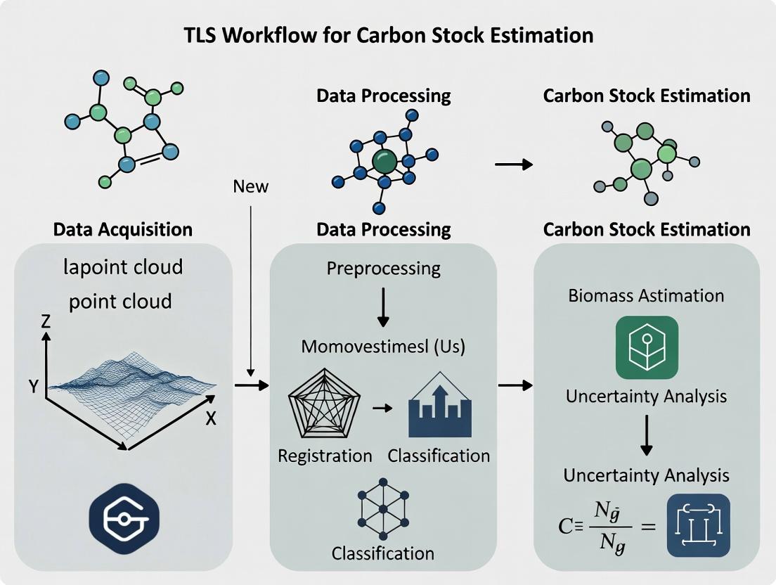
Visualized Workflows and Relationships

Title: End-to-End TLS Carbon Stock Workflow

Title: TLS as the Optimal Solution for Biomass

The Scientist's Toolkit: Research Reagent Solutions

Table 3: Essential Materials for TLS-Based Biomass Research

Item / Solution	Function / Purpose
Phase-Based or Time-of-Flight TLS Scanner (e.g., Faro Focus, RIEGL VZ-400)	Core instrument for capturing high-density, millimeter-accurate 3D point clouds of vegetation structure.
Calibrated Reference Spheres/Targets	High-contrast targets used as stable tie points for accurate co-registration of multiple scans in a plot.
Geodetic GNSS Receiver (e.g., Trimble, Leica)	Provides precise geolocation for scan positions, enabling plot georeferencing and longitudinal re-measurement.
Point Cloud Processing Software (e.g., CloudCompare, 3D Forest)	Open-source or commercial platform for registration, filtering, classification, and analysis of TLS data.
QSM Reconstruction Algorithm (e.g., TreeQSM, SimpleTree)	Specialized computational method to convert a tree point cloud into a volumetric cylinder model for biomass derivation.
Wood Density Database (e.g., Global Wood Density Database)	Provides the essential species-specific parameter (ρ) to convert geometric volume to dry mass.
High-Performance Computing Workstation	Necessary for handling large (>1 billion point) datasets and running computationally intensive QSM algorithms.

Within a thesis on TLS workflow for carbon stock estimation, understanding the fundamental operational principles of Terrestrial Laser Scanners (TLS) is critical. This document details the core technology and provides standardized protocols for capturing forest 3D structure, a primary input for allometric modeling and biomass calculation.

Core Operating Principles

A TLS is an active remote sensing instrument that emits laser pulses to measure distances to surfaces. The core principle is Light Detection and Ranging (LiDAR). The scanner calculates the distance to an object based on the time-of-flight (ToF) of a laser pulse or the phase shift of a modulated laser beam. By systematically rotating and scanning across a defined field-of-view, it captures millions of 3D points (a point cloud), where each point has X, Y, Z coordinates and often intensity (I) values.

Key System Components & Their Function

• Laser Emitter: Generates coherent, focused light pulses (typically in NIR, e.g., 905nm or 1550nm for eye safety).
• Scanning Mechanism (Mirror/Galvanometer): Deflects the laser beam across the scene.
• Receiver/Detector: Captures the backscattered light signal.
• Precise Timing Circuitry: Measures Time-of-Flight (ToF) with nanosecond accuracy.
• Internal/External Orientation System: Includes inclinometers, compasses, and high-resolution angular encoders to precisely define the beam's origin and direction.
• Control Unit & Data Storage: Manages operation and stores raw measurements.

Data Acquisition Workflow

Diagram Title: TLS Data Acquisition and Processing Workflow

Key Protocols for Capturing 3D Forest Structure

Protocol 1: Pre-Field Campaign Planning

Objective: Ensure optimal scanner setup and scan geometry for complete scene coverage.

• Site Selection: Define plot locations representative of forest structure (e.g., within permanent forest inventory plots).
• Scan Resolution Determination: Set angular resolution (e.g., 0.05° at 10m range yields ~8.7mm point spacing). Balance detail with file size and scan duration.
• Scan Position Planning: Design a network of scanner positions to minimize occlusions (e.g., plot center and 4 cardinal sub-positions). Use a "hairpin" or "cross" pattern.
• Target Placement: Plan for high-reflectivity, spherical targets (e.g., 6-10) placed stably throughout the plot for subsequent scan co-registration.

Protocol 2: Field Deployment & Scanning

Objective: Acquire high-quality, overlapping point clouds from multiple positions.

• Instrument Setup: Level and stabilize the TLS on a tripod. Record instrument height.
• Scanner Registration: For systems requiring it, establish a local coordinate system.
• Scan Execution: Initiate scan per planned resolution. A full dome scan (360° horizontal, 270-330° vertical) is standard. Record scan metadata.
• Target Scan: Perform a high-resolution scan of targets if they are not clearly resolved in the full scan.
• Position Iteration: Move TLS to the next pre-planned position, ensuring overlap in target visibility. Repeat steps 1-4.

Protocol 3: Post-Processing & Data Registration

Objective: Create a single, aligned, and clean point cloud of the entire plot.

• Data Transfer & Backup: Transfer raw data from scanner media.
• Target-Based Registration: Use specialized software (e.g., CloudCompare, Faro Scene, RiSCAN PRO) to identify identical target centers across scans and perform an iterative closest point (ICP) algorithm for fine alignment.
• Quality Control: Assess registration error. Root Mean Square (RMS) error should be < 6mm for structural analysis.
• Noise Filtering: Apply range-dependent noise filters and remove obvious outliers (e.g., flying birds, insects).
• Export Final Cloud: Export the registered point cloud in a standard format (e.g., .las, .laz, .pts).

Quantitative Performance Parameters of Typical TLS Systems

Table 1: Comparative Specifications of Common TLS Technology Types for Forestry

Parameter	Phase-Shift Scanner	Time-of-Flight (ToF) Scanner	Notes for Forest Applications
Typical Max Range	80m - 120m	500m - 2000m+	ToF better for open forests; Phase-shift sufficient for dense canopy.
Measurement Rate	500,000 - 2,000,000 pts/sec	10,000 - 100,000 pts/sec	High-rate phase-shift captures fine twigs and leaves.
Ranging Accuracy	1-5 mm	2-10 mm	Both sufficient for tree DBH and stem modeling.
Beam Divergence	0.1 - 0.5 mrad	0.3 - 1.0 mrad	Lower divergence yields finer detail on edges.
Eye Safety	Typically Class 1 (1550nm)	Often Class 3R (905nm)	Longer wavelength (1550nm) is inherently safer.
Primary Forestry Use	High-detail plot inventory, leaf area, understory	Large-scale transects, tall canopy profiling	Choice depends on plot size and structural detail required.

Table 2: Recommended Scan Parameters for Forest Carbon Stock Estimation

Scanning Variable	Recommended Setting	Rationale
Angular Resolution	0.02° - 0.08° (0.35 - 1.4 mrad)	Balances detail (fine branches) with manageable data volume.
Minimum Scan Positions per Plot	5 (Center + 4)	Drastically reduces occlusion, capturing >95% of stem surface.
Targets per Scan	≥ 4 common targets	Ensures robust registration. More targets improve accuracy.
Scan Duration per Position	5 - 15 minutes	Varies with resolution and field of view.

The Scientist's Toolkit: Essential Research Reagents & Materials

Table 3: Key Materials for TLS Forest Inventory Field Campaign

Item	Category	Function in TLS Workflow
Terrestrial Laser Scanner	Instrument	The primary data acquisition tool. Must be selected based on range, speed, and accuracy needs (see Table 1).
High-Stability Tripod	Hardware	Provides a stable, level platform for the scanner, minimizing noise and drift during scan.
Spherical Targets (e.g., 140mm)	Registration Aid	High-contrast, geometrically defined objects placed in the scene to provide reference points for aligning multiple scans.
Target Mounting Kit (Poles, Clamps)	Hardware	Allows for secure and precise placement of spherical targets at various heights within the plot.
Invar Bar or Calibrated Baseline	Calibration Tool	Used for periodic field validation of scanner distance measurement accuracy.
Ruggedized Field Laptop/Tablet	Data Management	For initial data checks, control of some scanners, and backup in the field.
Portable Power Supply	Power	Ensures continuous scanner operation in remote plots without grid power.
Digital Inclinometer/Compass	Supplementary Data	Provides independent measurement of scanner orientation for coarse alignment or validation.
Field Notebook & Camera	Metadata Collection	Documents plot conditions, target layouts, and any anomalies during scanning.

Terrestrial Laser Scanning (TLS) provides a non-destructive, high-resolution method for estimating above-ground biomass (AGB) and carbon stocks in forest ecosystems. This pipeline, conceptualized within a thesis on quantitative carbon stock estimation, translates raw 3D point clouds into actionable carbon metrics. The protocol is critical for researchers in environmental science, climate change mitigation, and underpins ecological models used in broader biogeochemical research.

Core Conceptual Workflow

The end-to-end pipeline involves sequential stages from field planning to carbon calculation.

TLS to Carbon Core Workflow Pipeline

Detailed Experimental Protocols

Protocol: Field Site Acquisition with TLS

Objective: Capture complete, high-quality 3D point clouds of a forest plot. Materials: See Reagent Solutions Table. Procedure:

• Plot Establishment: Delineate a fixed-area plot (e.g., 40m x 40m). Georeference plot corners with RTK-GPS (≤2 cm accuracy).
• Scanner Setup: Position TLS on a stable tripod at plot center. Level the instrument. Measure scanner height.
• Scan Registration: Place at least 4 high-reflectivity targets (spheres/checkboards) around the plot, ensuring inter-visibility between scan positions.
• Acquisition: Perform a 360° horizontal and 270° vertical scan at high resolution (e.g., point spacing at 10m: 6.3mm). Use multi-scan registration by moving scanner to sub-positions (e.g., plot corners) and repeating, keeping targets fixed.
• Metadata Log: Record scanner model, resolution, date, time, and weather conditions.

Protocol: Point Cloud Pre-processing & Alignment

Objective: Generate a single, clean, and aligned point cloud dataset. Software: CloudCompare, FARO SCENE, or R lidR package. Procedure:

• Import & Target Registration: Import all scans. Manually or automatically identify target centers. Perform target-based coarse registration.
• Fine Registration: Apply Iterative Closest Point (ICP) algorithm on overlapping natural features for sub-cm alignment error.
• Noise Filtering: Apply statistical outlier removal (e.g., filter points with mean distance > 1 standard deviation from 50 nearest neighbors).
• Normalization: Use a ground classification algorithm (e.g., Cloth Simulation Filter) to identify terrain. Subtract ground elevation to create a normalized point cloud (nPC) with heights above ground.

Protocol: Quantitative Structure Modeling (QSM)

Objective: Convert the nPC into quantitative tree architecture models. Software: TreeQSM (MATLAB), SimpleTree (C++), or compuTree. Procedure:

• Stem Detection & Segmentation: Apply a clustering algorithm (e.g., DBSCAN) to isolate individual trees. Use region-growing algorithms to separate stem from branches.
• Cylinder Fitting: Fit a series of overlapping cylinders to the stem and branch point clusters. The algorithm minimizes the difference between cylinder surface and points.
• Model Validation: Manually verify a subset (e.g., 20 trees). Compare QSM-derived Diameter at Breast Height (DBH) with field-measured DBH. Calibrate segmentation parameters until RMSE < 2 cm.

Protocol: Volume to Carbon Stock Estimation

Objective: Calculate above-ground biomass (AGB) and convert to carbon stock. Procedure:

• Volume Calculation: Sum the volumes of all cylinders in the QSM for each tree: V = Σ (π * radius² * cylinder height).
• Biomass Estimation:
  • Option A (Allometric): Use QSM-derived DBH and species-specific allometric equations (e.g., AGB = a * DBH^b).
  • Option B (Volume-Based): Multiply total wood volume by wood density (species-specific) and a biomass conversion factor: AGB = V * ρ * BCF.
• Carbon Stock Calculation: Multiply AGB by the default carbon fraction (0.47 for IPCC guidelines): Carbon = AGB * 0.47.
• Uncertainty Propagation: Propagate errors from volume reconstruction, wood density, and allometric models using Monte Carlo simulation.

Data Presentation

Table 1: Comparison of TLS-Derived Metrics vs. Traditional Field Inventory

Metric	TLS-Derived Mean (±SD)	Traditional Field Mean (±SD)	Relative Difference	Key Advantage of TLS
DBH (cm)	32.4 (±15.2)	32.1 (±15.0)	+0.9%	Non-destructive, captures asymmetry
Tree Height (m)	18.7 (±8.3)	17.9 (±8.1)*	+4.5%	Objective, avoids crown occlusion bias
Stem Volume (m³)	1.85 (±2.1)	1.72 (±1.9)	+7.6%	Direct 3D measurement, no allometry needed
Plot AGB (Mg/ha)	245.5 (±45)	230.1 (±52)	+6.7%	Captures non-stem biomass components

Field height often underestimated due to canopy overlap. *Traditional volume/AGB relies on allometric models introducing uncertainty.

The Scientist's Toolkit: Research Reagent Solutions

Table 2: Essential Materials for TLS Carbon Workflow

Item	Function & Specification
Terrestrial Laser Scanner	High-accuracy phase-based or time-of-flight scanner (e.g., RIEGL VZ-400, FARO Focus). Key specs: <5mm accuracy, >1km range, full dome capture.
Registration Targets	High-reflectivity spheres or checkerboard targets. Crucial for precise co-registration of multiple scans in the field.
RTK-GPS System	Provides geospatial context and accurate plot corner locations (≤2 cm accuracy). Enables integration with aerial LiDAR or satellite data.
Stable Survey Tripod	Heavy-duty tripod with tribrach for stable, level scanner setup, minimizing vibration-induced noise.
Processing Software Suite	e.g., CloudCompare (open-source), FARO SCENE (vendor), R lidR & TreeQSM for analysis. For algorithm development: MATLAB, Python (Open3D, PyVista).
Field Computer/Tablet	Ruggedized device for data backup, scanner control, and metadata logging on-site.
Wood Density Database	Species-specific wood density values (e.g., from Global Wood Density Database). Critical for volume-to-biomass conversion.
Validation Equipment	Diameter tape, clinometer, or ultrasonic height gauge for collecting ground-truth data to validate TLS metrics.

Carbon Stock Calculation Pathway

Application Notes

Terrestrial Laser Scanning (TLS) provides high-resolution, three-dimensional data critical for quantifying forest structure. This non-destructive method enables precise estimation of Above-Ground Biomass (AGB), a fundamental metric for carbon accounting and climate change mitigation research. TLS-derived metrics, such as stem volume and canopy architecture, serve as input for allometric models that convert structural data into carbon stock estimates (units: Mg C ha⁻¹). This approach reduces uncertainty compared to traditional field surveys, enhancing the accuracy of national greenhouse gas inventories and ecological forecasts.

In forest ecology, TLS captures forest heterogeneity, gap dynamics, and habitat structure at unprecedented detail, supporting research on biodiversity, succession, and disturbance recovery. For climate change research, TLS time-series data track carbon flux dynamics, monitor forest health under climate stress, and validate remote sensing products from LiDAR and satellites, scaling plot-level findings to landscapes.

Table 1: Comparative Analysis of Carbon Estimation Methods

Method	Spatial Scale	Key Measured Parameter	Estimated Accuracy (vs. Destructive Harvest)	Primary Application Context
Destructive Harvest	~0.04 ha (plot)	Dry mass of all components	100% (benchmark)	Calibration; rare due to cost & destructiveness
Field Allometry	~0.1 ha (plot)	Diameter at Breast Height (DBH), Height	±20-30% (varies by model/forest type)	National forest inventories; ecological studies
Terrestrial Laser Scanning (TLS)	~1 ha (plot)	3D point cloud; stem volume, canopy metrics	±10-20% (when properly calibrated)	High-accuracy carbon accounting; model validation
Airborne LiDAR (ALS)	100s - 1000s ha	Canopy height, cover profiles	±20-40% (requires ground calibration)	Landscape-scale mapping; regional carbon stocks
Satellite (e.g., GEDI, ICE-Sat-2)	Continental/Global	Canopy height, structure profiles	±40-60% (requires robust calibration)	Global carbon budget; biome-level change detection

Table 2: TLS-Derived Metrics for Ecological and Climate Studies

Metric	Calculation from TLS Point Cloud	Ecological Relevance	Carbon Accounting Utility
Stem Diameter (DBH)	Cylinder fitting or convex hull at 1.3 m height	Tree growth, size class distribution	Direct input for allometric biomass equations
Tree Height	Difference between highest canopy point and local ground	Canopy stratification, competition	Improves allometric model precision
Stem Volume	Quantitative Structure Model (QSM) voxelization	Stand productivity, woody biomass	Converts to mass using wood density (less model reliance)
Canopy Cover	Gap fraction analysis from zenith angles	Light interception, habitat	Informs growth models and carbon uptake estimates
Leaf Area Index (LAI)	Inversion of gap probability	Ecosystem productivity, water use	Constrains parameters in ecosystem process models
Crown Rugosity	3D complexity from surface roughness	Biodiversity proxy, niche diversity	Correlates with total plot biomass and microclimate

Experimental Protocols

Protocol 1: TLS Field Campaign for Carbon Stock Estimation

Objective: To acquire spatially comprehensive TLS data from a forest plot for constructing 3D models and estimating AGB. Materials: Terrestrial Laser Scanner (e.g., RIEGL VZ-400, Faro Focus), high-capacity batteries, calibrated reflectors/targets, GNSS receiver (optional for georeferencing), clinometer, field computer, inventory tags. Pre-Survey Planning:

• Define plot (typically 1-ha circular or rectangular). Establish plot center and mark boundaries.
• Design scanner positions to minimize occlusion. A minimum of 5 positions per hectare is recommended, including the plot center and four cardinal sub-plot centers. Field Procedure:
• Set up scanner on a stable tripod at the first position. Ensure the scanner is level.
• Place 4-5 reference spheres or checkerboard targets around the plot, ensuring they are visible from multiple scanner positions.
• Perform a 360-degree scan with high resolution settings (e.g., 0.03° angular step at 10 m). For a RIEGL VZ-400, use "Multi Scan" mode with the following typical settings: Scan speed: 3 (medium-high); Vertical and Horizontal resolution: 0.03°; Range: Up to 350m for forest settings.
• Record the scan position and target coordinates. Move to the next pre-planned position and repeat, ensuring at least 3 targets overlap between consecutive scans.
• Perform a field inventory: Measure DBH, species, and map tree positions for all trees >10 cm DBH within the plot. This data is critical for validation. Data Processing Workflow: See Diagram 1.

Protocol 2: Quantitative Structure Model (QSM) Generation for Volume Estimation

Objective: To convert the registered point cloud into a volumetric tree model for direct biomass computation. Software: 3D Forest, Computree, or standalone algorithms (e.g., SimpleTree). Input Data: Co-registered, cleaned plot point cloud from Protocol 1. Procedure:

• Individual Tree Segmentation: Use a clustering algorithm (e.g., Euclidean distance clustering) or a canopy height model (CHM)-based method to isolate points belonging to individual trees.
• Stem and Branch Detection: Apply a stem detection algorithm to identify the main trunk. Algorithms typically search for vertically contiguous points with cylindrical properties.
• Cylinder Fitting: Fit a series of overlapping cylinders along the detected stem and branches. The algorithm (e.g., RANSAC) iteratively finds the best-fit cylinder for a cluster of points, moving upward and outward from the trunk.
• Model Reconstruction: Connect the fitted cylinders to create a coherent, watertight branch network—the QSM.
• Volume Calculation: Calculate the volume of each cylinder (π * r² * h). Sum all cylinder volumes to obtain total tree woody volume.
• Biomass Conversion: Multiply total woody volume (m³) by species-specific wood density (kg/m³, from global databases like Global Wood Density Database) to get mass. Convert to carbon mass using a default factor of 0.47–0.50 g C per g dry mass.

Mandatory Visualization

TLS Data Processing Workflow for Carbon Stocks

From Point Cloud to Tree Carbon Mass via QSM

The Scientist's Toolkit: Research Reagent Solutions & Essential Materials

Item Name	Category	Function in TLS Carbon Workflow
RIEGL VZ-400/VZ-600	TLS Instrument	Time-of-flight laser scanner. Provides high-accuracy, long-range (>350m) point clouds. Essential for capturing dense forest structure.
Faro Focus Premium	TLS Instrument	Phase-shift laser scanner. Offers very high scan speed and resolution for detailed stem and canopy architecture.
Spectralon Targets	Field Calibration	High-reflectivity, Lambertian surfaces. Used as stable reference points for co-registering multiple scans.
Cyclone REGISTER 360	Software	Point cloud registration and processing suite. Aligns multiple scans using target- or cloud-based registration.
3D Forest Software	Analysis Software	Integrated platform for TLS point cloud analysis, including tree detection, DBH extraction, and simple volume modeling.
SimpleTree (C++ Library)	Algorithm	Open-source tool for automatic reconstruction of tree models (QSM) from point clouds, enabling volume estimation.
Global Wood Density Database	Reference Data	Curated repository of species-specific wood density values. Critical for converting tree volume to dry biomass.
RANSAC Algorithm	Computational Method	Random Sample Consensus. Core algorithm for robust geometric primitive (e.g., cylinder) fitting in noisy point clouds.
Field Inventory Kit (Caliper, Tape, Tags)	Validation Tool	Used for ground-truth measurement of DBH, height, and species. Essential for validating and calibrating TLS-derived metrics.
R Package 'lidR'	Analysis Software	Open-source environment for processing LiDAR data, including tree segmentation, metric extraction, and spatial analysis.

This document details the hardware foundations for Terrestrial Laser Scanning (TLS) within a comprehensive thesis workflow for forest carbon stock estimation. Precise, three-dimensional quantification of above-ground biomass (AGB) relies on the accurate selection and application of TLS hardware. These Application Notes outline scanner types, specifications, and protocols to inform researchers, scientists, and professionals on optimal data acquisition strategies for ecological structural analysis.

TLS Scanner Types for Ecological Applications

Terrestrial Laser Scanners are categorized primarily by their ranging principle, which dictates their suitability for forest structural surveys.

Time-of-Flight (ToF) Scanners: Emit a laser pulse and measure the time for its reflection to return. Effective for long-range measurements in complex, open forests. Phase-Shift (PS) Scanners: Modulate laser beam amplitude and measure the phase difference between emitted and reflected waves. Typically faster and more precise at shorter ranges. Triangulation-based Scanners: Use a laser stripe and a camera at a known baseline. Limited to very short ranges, less common for field ecology.

Quantitative Scanner Specification Comparison

Table 1: Key TLS Scanner Specifications for Carbon Stock Estimation Research (Representative Models)

Scanner Type	Example Model	Ranging Principle	Effective Range (m)	Ranging Accuracy (mm)	Scan Speed (points/sec)	Beam Divergence (mrad)	Key Ecological Application Suitability
Long-Range ToF	RIEGL VZ-400i	Time-of-Flight	1.5 – 800	3 @ 100 m	Up to 500,000	0.35	Large plot, open forest, long-range trunk detection
Mid-Range PS	FARO Focus Premium	Phase-Shift	0.6 – 350	±1.0 @ 10 m	Up to 2,000,000	0.19	High-detail understory, plot-level stem & branch mapping
Hybrid ToF	Leica RTC360	Time-of-Flight	0.6 – 130	1.1 mm @ 10 m + 10 ppm	Up to 2,000,000	0.3	Rapid, high-resolution plot scans with integrated imagery
Portable/Mobile	GeoSLAM ZEB Horizon	Simultaneous Localization & Mapping (SLAM)	Up to 100	1 – 3 cm typical	300,000	N/A	Under-canopy transects, difficult terrain, no fixed station

Data compiled from manufacturer specifications (2024). Accuracy is range-dependent; consult specific datasheets.

Core Experimental Protocols for TLS Carbon Workflow

Protocol 3.1: Multi-Scan Station Plot Survey for Volume Reconstruction

Objective: Capture a complete, occlusion-minimized 3D point cloud of a fixed-area forest plot (e.g., 40m x 40m). Materials: TLS unit (e.g., FARO or RIEGL), tripod, calibration targets/spheres, external battery, field computer, GNSS receiver (optional for geo-referencing). Procedure:

• Pre-Survey Planning: Define plot corners. Plan 6-10 scan positions in a grid or offset pattern, ensuring line-of-sight to multiple registration targets from each position.
• Target Placement: Distribute 4-6 spherical targets or checkerboards throughout the plot, ensuring stability and visibility.
• Scanning: Level and setup scanner at first position. Perform a preview scan. Execute a full 360°x300° high-resolution scan (e.g., 1/4 or 1/8 resolution at 10m).
• Registration: Ensure ≥3 targets are visible between consecutive stations. Record target centers if required for manual registration.
• Iterate: Move to next pre-planned station, repeat. Overlap coverage >30%.
• Data Transfer & Backup: Securely transfer raw scan (.fls, .sd) and project files daily.

Protocol 3.2: SLAM-based Understory and Transect Survey

Objective: Rapidly capture forest structure along a transect or in dense understory where tripod setup is impractical. Materials: Wearable or handheld SLAM scanner (e.g., GeoSLAM ZEB), protective case, pre-marked start/stop loop closure points. Procedure:

• System Warm-up: Initialize the scanner in an open area for 30-60 seconds as per manufacturer guidelines.
• Loop Closure Definition: Define start point (e.g., a distinctive tree). Plan a walk route that returns to within 1-2m of this point to close the loop.
• Data Acquisition: Walk at a steady pace (~0.8-1.0 m/s), avoiding sharp lateral movements. Point the scanner towards stems and canopy. Maintain a consistent “figure-of-eight” motion when stationary to improve point cloud density.
• Loop Closure: End the scan near the start point. Post-processing software uses loop closure to correct drift.
• Multiple Passes: For enhanced detail, walk the same transect in orthogonal directions.

Visualization of TLS Carbon Workflow

TLS to Carbon Stock Estimation Workflow

TLS Scanner Selection Logic for Ecology

The Scientist's Toolkit: Research Reagent Solutions

Table 2: Essential Non-Hardware Materials for TLS Field Campaigns

Item	Function in TLS Carbon Research
Spherical/Checkerboard Targets	High-contrast objects for precise co-registration of multiple scan stations.
High-Capacity Field Battery	Powers TLS unit for full-day operation (>8 hrs) remote from grid power.
Ruggedized Field Laptop & SSD	For data verification, basic pre-processing, and secure backup in the field.
Precision Inclinometer/Tripod	Ensures leveling of scanner head to minimize systematic error in data.
Field Calibration Panel	Used for periodic radiometric calibration, ensuring intensity value consistency.
GNSS Receiver (RTK Grade)	Provides precise geo-referencing of scan data for multi-temporal studies.
Stem Diameter Tape & Clinometer	Traditional measurement tools for validating TLS-derived metrics (DBH, height).
Data Logbook (Waterproof)	To record scan positions, target maps, and environmental conditions.

A Step-by-Step TLS Workflow: From Field Deployment to Carbon Stock Calculation

Within the comprehensive workflow for terrestrial laser scanning (TLS)-based carbon stock estimation, pre-field planning is the critical first phase that determines the validity, efficiency, and scalability of the entire research project. This phase involves the deliberate design of a sampling strategy and plot layout to ensure that collected point clouds are statistically representative, minimize occlusion, and facilitate accurate dendrometric extraction. This protocol details the application notes for this foundational stage.

Core Quantitative Considerations for Strategy Design

Table 1: Key Quantitative Parameters for TLS Plot Design

Parameter	Typical Range / Value	Rationale & Impact
Minimum Plot Radius	≥ 25 m (forests)	Ensures inclusion of sufficient trees for representative statistics and reduces edge effects.
Scan Resolution (Angular)	0.02° - 0.1° (0.35 - 1.7 mrad)	Balances point density (e.g., > 10 pts/cm² on trunk at 25m) with scan duration and data volume.
Number of Scan Positions per Plot	1 (Single-scan) to 5+ (Multi-scan)	Increases completeness of tree models. ≥4 positions (center + subplot corners) is common for biomass studies.
Subplot Sampling Intensity	10-30% of total area	For nested designs, TLS scans in subplots enable calibration with destructive or traditional mensuration.
Distance Between Scan Positions	10-20 m	Optimizes angular perspective change to reduce occlusion while maintaining registration accuracy.

Table 2: Comparison of Common TLS Sampling Strategies

Strategy	Description	Pros	Cons	Best For
Single-Scan Plot	One scan at plot center.	Fast, simple registration.	High occlusion, poor stem & crown reconstruction.	Rapid inventory, stem mapping.
Multi-Scan Center	Multiple scans at plot center (different heights/tilts).	Better vertical coverage.	Does not mitigate horizontal occlusion.	Understory assessment.
Multi-Scan Polygon	Scans at plot center and vertices (e.g., 5 scans).	Excellent coverage, robust DBH & volume models.	Time-consuming, complex registration.	High-accuracy biomass estimation.
TLS Transect	Sequential scans along a line.	Efficient for linear features.	Complex plot definition, edge effects.	Riparian zones, ecological gradients.

Experimental Protocols

Protocol 1: Designing a Multi-Scan Plot for Carbon Stock Estimation

Objective: To establish a permanent plot layout that maximizes 3D structural capture for individual tree detection and volume modeling.

Materials: See "The Scientist's Toolkit" below.

Procedure:

• Site Assessment: Using pre-existing data (e.g., aerial imagery, forest inventory maps), identify homogeneous forest strata. Define target plot locations to represent these strata.
• Plot Demarcation: In the field, establish a circular or square main plot (e.g., 30m radius). Mark the georeferenced center point (P0) permanently.
• Scan Position Layout: Implement a 5-scan layout:
  • Position P0 at plot center.
  • Position P1-P4 at 10-15m from center at 90° intervals (N, E, S, W) or at the corners of a square subplot.
• Scanning Protocol at Each Position:
  • Level and mount the TLS on tripod. Measure height of scanner's axis.
  • Set scan resolution to 0.05° (approx. 0.87 mrad) for full-dome scans.
  • For each scan, use high-visibility targets (spheres/checkboards) placed in stable, mutually visible locations to aid subsequent co-registration. A minimum of 3 targets must be visible from any two adjacent scan positions.
  • Perform the scan, ensuring no movement occurs during acquisition.
• Ancillary Data Collection: Within the same plot, conduct complementary measurements:
  • Destructive Calibration Subplot: In a nested subplot (e.g., 10m radius), tag, measure DBH, and identify all trees. A subset may be felled for direct biomass measurement and allometric model calibration.
  • Traditional Mensuration: For all trees >10cm DBH in the main plot, record species, DBH, height (using hypsometer), and crown position.

Protocol 2: Registration and Data Quality Check

Objective: To align multiple scans into a single, coherent point cloud and verify data integrity.

Procedure:

• Target-Based Registration: In processing software (e.g., Cyclone, CloudCompare), manually or automatically identify the centers of the reference targets in each scan. Use these matching points to compute the rigid transformation (rotation, translation) that aligns all scans to a common coordinate system (e.g., centered on P0).
• Fine Registration: Apply an Iterative Closest Point (ICP) algorithm on overlapping natural features to refine alignment, using the target-based registration as an initial guess.
• Quality Control: Quantify registration error as the root mean square error (RMSE) of target residuals. Accept if < 1 cm. Visually inspect merged point cloud for ghosting or misalignment artifacts.
• Occlusion Mapping: Analyze the final merged point cloud to identify persistent "data shadows" (e.g., behind very large trees). Document these areas as potential sources of uncertainty.

Visualized Workflows

TLS Pre-Field & Field Workflow for Plot Setup

Multi-Scan Plot Layout with Calibration Subplot

The Scientist's Toolkit

Table 3: Essential Research Reagent Solutions for TLS Plot Planning

Item	Function & Specification
Phase-Based TLS Scanner	High-accuracy distance measurement (e.g., ±2 mm). Preferred for forestry over time-of-flight for faster acquisition. Example: Faro Focus series.
Geodetic-Grade GNSS Receiver	Provides precise georeferencing (cm-level accuracy) for plot corners and scan positions, enabling multi-plot integration and repeat surveys.
High-Visibility Registration Targets	Spherical (preferred) or planar checkboard targets. Act as known reference points for accurate co-registration of multiple scans.
Dendrometric Field Kit	Diameter tape, clinometer or hypsometer, total station for layout. Provides ground-truth data for validating TLS-derived metrics (DBH, height).
Ruggedized Field Computer/Tablet	For real-time data logging, viewing preliminary scans, and managing field metadata.
Point Cloud Processing Software	Commercial (e.g., Leica Cyclone, Faro Scene) or open-source (CloudCompare, R lidR). Used for registration, visualization, and analysis.
Allometric Model Database	Species-specific or generic equations (e.g., Jenkins, Chave) to convert TLS-derived tree volumes to dry biomass and carbon stock.

This protocol, framed within a broader thesis on Terrestrial Laser Scanning (TLS) workflow for carbon stock estimation research, details the standardized procedures for field deployment of TLS systems. Consistent execution is critical for acquiring high-fidelity 3D point clouds for quantitative structure modeling (QSM) and biomass estimation.

1. Pre-Deployment Site Preparation & Planning Objective: Ensure logistical and environmental readiness for efficient scanning. Protocol:

• Desktop Study: Utilize GIS software to analyze site topography, access routes, and potential obstructions using satellite imagery and digital terrain models.
• Scan Planning: Based on research plot dimensions (e.g., 40m x 40m or 1ha), determine optimal scan locations (≥4 per plot) to minimize occlusion. Positions should offer clear lines of sight to all trees, with overlap between scans >30%.
• Target Placement Strategy: Plan for the deployment of artificial targets (e.g., sphere/checkerboard) at stable locations throughout the plot. A minimum of 4 targets must be visible from any two adjacent scan positions for robust registration.
• Safety & Permissions: Secure necessary field permits and conduct a site-specific risk assessment.

2. Scanner Setup & Calibration Protocol Objective: Achieve optimal instrument configuration for accurate data capture. Protocol:

• Power & Environment: Ensure all batteries are fully charged. Allow the scanner to acclimate to ambient temperature if transported in a conditioned vehicle.
• Hardware Assembly: Mount the TLS (e.g., RIEGL VZ-400, Faro Focus) securely on a stable tripod. Level the instrument using the integrated bubble level.
• System Initialization: Power on the scanner and connected controller (tablet/laptop). Establish a stable communication link.
• In-Situ Calibration Check: Perform a low-resolution pre-scan. Visually inspect the point cloud for obvious anomalies (e.g., striping, distortions) which may indicate the need for service calibration.

3. Scanning & Target Deployment Protocol Objective: Capture comprehensive plot geometry with embedded reference points. Protocol:

• Scan Parameter Configuration: Set scan resolution based on plot size and stem density. Recommended parameters are summarized in Table 1.
• Target Deployment: Place calibrated targets (≥6 per plot) on stable tripods or firmly attached to stakes. Ensure they are distributed around and within the plot, at varying heights where possible.
• Scan Execution: Initiate scan from the first pre-planned position. Monitor progress for interruptions (e.g., moving vegetation, people). Repeat for all n scan positions.
• Metadata Logging: For each scan, manually record: Scan ID, GPS coordinates (if available), tilt/tilt compensator status, and environmental notes (wind, precipitation).

Table 1: Recommended TLS Scan Parameters for Forest Inventory

Plot Size (ha)	Angular Resolution	Range Noise Filter	Estimated Scan Time per Position	Key Rationale
0.04 - 0.25	0.02° - 0.035°	Low/Medium	8 - 15 minutes	High detail for QSM; balance of noise and capture time.
>0.25 - 1.0	0.035° - 0.05°	Medium	5 - 10 minutes	Maintains stem detection at longer ranges; efficient coverage.

4. Multi-Scan Registration Protocol Objective: Accurately align all individual scans (n) into a single, coherent plot point cloud. Protocol:

• Target-Based Registration (Primary Method): a. In proprietary software (e.g., RIEGL RISCAN PRO, Leva Cyclone), import all scans. b. For each scan, manually or automatically detect the 3D centers of all visible targets. c. Use a least-squares adjustment algorithm to compute the transformation parameters (3D translation & rotation) that minimize the distances between corresponding target centers across scans. d. Assess registration error by examining the residual misalignment for each target. The mean error should be ≤ 5 mm.
• Cloud-to-Cloud Refinement (Optional): a. Apply an Iterative Closest Point (ICP) algorithm to the target-registered point cloud. b. Use this only on stable surfaces (e.g., large stems, ground) to fine-tune alignment. Exclude foliage and branches.
• Quality Control: Visually inspect the merged point cloud for duplication (ghosting) or misalignment of stems. Check that the plot boundaries are seamless.

5. Best Practices for Multi-Scan Campaigns

• Temporal Consistency: For repeat campaigns (e.g., annual biomass growth), permanently mark scan positions and target locations with buried stakes or monuments for exact reoccupation.
• Data Management: Immediately back up raw scan data (.sd, .fls, .pts) and registration projects from the field controller to secured storage.
• Foliage Considerations: Deciduous plots should be scanned during leaf-off periods for improved stem visibility, where research objectives allow.

Diagram: TLS Field-to-Data Workflow

The Scientist's Toolkit: Essential TLS Field Materials

Item / Reagent Solution	Function in Protocol
Terrestrial Laser Scanner (e.g., RIEGL, Leica, Faro)	Core instrument for emitting laser pulses and measuring return signals to create 3D point clouds.
Calibrated Spherical/Checkerboard Targets	High-contrast, geometrically defined objects placed in the scene to provide known reference points for accurate scan alignment.
Survey-Grade Tripod & Tribrach	Provides a stable, level platform for the scanner, minimizing vibration and ensuring consistent scanning geometry.
Field Controller (Ruggedized Tablet/Laptop)	Hosts scanner control software for parameter configuration, scan execution, and real-time data preview.
High-Capacity Batteries & Power Bank	Ensures uninterrupted operation of scanner and controller during extended field sessions.
Inclination Sensor / Tilt Compensator (Integrated)	Measures and corrects for minor tripod tilt, improving the vertical alignment of individual scans.
Digital Camera (Often Integrated)	Captures high-resolution hemispheric images for colorizing point clouds (RGB attributes).
GNSS Receiver (Optional but Recommended)	Provides georeferenced coordinates for scan positions, facilitating multi-plot and multi-temporal studies.
Dense Foam Balls / Signalization Tape	Used to temporarily mark small branches or foliage during scanning for tracking movement between scans.

Application Notes

Within a Terrestrial Laser Scanning (TLS) workflow for carbon stock estimation, the initial data processing stage is critical for transforming raw, unorganized 3D point measurements into a clean, accurate, and spatially coherent digital model of a forest plot. This stage directly impacts the accuracy of subsequent feature extraction (e.g., stem detection, DBH measurement) and biomass allometric equations. Errors introduced here propagate through the entire analysis, compromising carbon stock quantification.

Key Challenges: Raw TLS data from forest environments contain inherent noise from system error, wind-induced plant movement, occlusion (leading to data gaps), and non-target objects (e.g., understory vegetation, animals). Scans from multiple stations require precise alignment (registration) to create a complete 3D representation.

Quantitative Impact of Processing Stages: The following table summarizes typical data volume changes and error metrics through Stage 1 processing for a 1-hectare forest plot.

Table 1: Quantitative Impact of Stage 1 Processing on TLS Forest Data

Processing Step	Typical Input Data Volume	Typical Output Data Volume	Key Error Metric Targeted	Target Reduction/Accuracy
Multi-Station Registration	4-8 separate scans (~2-4 billion points)	1 coalesced cloud (~2-4 billion points)	Registration Error (RMSE)	< 0.01 m RMSE between scan ties
Outlier & Noise Removal	Coalesced cloud (~2-4 B points)	Cleaned cloud (~1.5-3.5 B points)	Proportion of spurious points	Removal of 5-20% of points as noise
Downsampling / Uniforming	Cleaned cloud (~1.5-3.5 B points)	Analysis-ready cloud (~0.5-1.5 B points)	Point density variance	Uniform density of ~1000 pts/m²

Experimental Protocols

Protocol 2.1: Target-Based Multi-Scan Registration

Objective: Precisely align multiple TLS scans (from different sensor positions) into a single, globally consistent coordinate system using artificial targets.

• Pre-Survey Target Placement: Before scanning, strategically place at least 4 high-contrast spherical targets throughout the plot, ensuring each is visible from a minimum of 3 scan positions.
• Scan Acquisition: Perform TLS scans from all planned positions, capturing the entire plot and all targets.
• Target Center Extraction: For each scan, automatically or manually identify each target. Use sphere-fitting algorithms to compute the precise 3D center coordinates of each target within the scan's local coordinate system.
• Correspondence & Transformation: Establish correspondences between identical targets across scans. Use a least-squares optimization (e.g., Iterative Closest Point algorithm variant) to compute the optimal rigid-body transformation (rotation & translation) that minimizes the distance between corresponding target centers.
• Validation: Check the Root Mean Square Error (RMSE) of target alignment post-registration. If RMSE > 0.01 m, inspect and correct target correspondence errors, then re-compute.

Protocol 2.2: Statistical Outlier Removal for Noise Reduction

Objective: Remove non-structural, sparse noise points caused by dust, flying insects, or beam divergence without smoothing fine structural details.

• Neighborhood Analysis: For every point in the (registered) cloud, compute the mean distance (d_mean) to its k nearest neighbors (e.g., k=20).
• Distribution Modeling: Compute the global mean (µ) and standard deviation (σ) of all d_mean values across the entire point cloud.
• Thresholding & Filtering: For each point, if its d_mean > µ + (n × σ), classify it as an outlier. A typical multiplier n ranges from 1.0 to 2.0, depending on noise level.
• Removal: Delete all points classified as outliers. The remaining point cloud retains dense clusters (true surfaces) while removing isolated, spurious points.

Protocol 2.3: Voxel-Grid Downsampling for Data Uniformity

Objective: Reduce data volume and create a more uniform point density to speed up subsequent processing, while preserving the overall shape and structural metrics.

• Define Voxel Size: Select a voxel (3D cube) edge length based on desired final point density and structural fidelity. For tree stems, a 0.01-0.02 m voxel is common.
• Partition Point Cloud: Subdivide the 3D space of the point cloud into a grid of voxels at the specified size.
• Point Reduction per Voxel: For each voxel that contains points, compute the centroid (geometric center) of all points within it.
• Replacement: Replace all points inside the voxel with the single centroid point. This reduces density in over-sampled areas while maintaining under-sampled areas.

Visualization: Stage 1 Workflow Diagram

Title: TLS Stage 1 Data Processing Workflow

The Scientist's Toolkit: Key Research Reagents & Materials

Table 2: Essential Materials for TLS Data Processing Stage 1

Item	Function in Protocol	Specification / Note
High-Contrast Spherical Targets	Acts as reference points for precise multi-scan registration.	Typically 100-200mm diameter spheres with matte finish. Bright color (e.g., orange) for automatic detection.
Target-Centroid Extraction Software	Identifies targets in scans and calculates their precise 3D center coordinates.	Often built into scanner manufacturer's software (e.g., Leva Cyclone, FARO SCENE).
Iterative Closest Point (ICP) Algorithm	Core computational engine for finding the optimal transformation to align two point clouds.	Implemented in libraries like Point Cloud Library (PCL), CloudCompare, Open3D.
Statistical Outlier Filter	Algorithm to remove sparse, isolated noise points based on local point density statistics.	Requires tuning of 'k-neighbors' and 'standard deviation multiplier' parameters.
Voxel-Grid Downsampling Filter	Algorithm to reduce point density uniformly while preserving macroscopic shape.	Key parameter is voxel leaf size, balancing data reduction and detail loss.
Georeferencing Equipment (Optional)	For tying the TLS model to real-world coordinates.	Total Station or High-precision GNSS to survey target positions in a geographic CRS.

Application Notes

Following the initial point cloud acquisition and preprocessing in a Terrestrial Laser Scanning (TLS) workflow for carbon stock estimation, the segmentation and classification stage is critical for attributing biomass components to 3D points. This stage directly influences the accuracy of subsequent wood volume and leaf area calculations, which underpin allometric modeling for carbon stocks. Current methodologies leverage machine learning, leveraging geometric and radiometric features derived from the point cloud itself.

Key Quantitative Performance Metrics of Contemporary Methods:

Method Category	Algorithm/Approach	Reported Accuracy (Overall)	Stem Precision	Branch Precision	Foliage Precision	Reference Year
Traditional Feature-Based	Multi-Scale Dimensionality Classification	85-92%	94-98%	80-87%	82-90%	2022
Deep Learning (DL)	PointNet++ with Component-Specific Weights	93-96%	98%	89-92%	91-95%	2023
Ensemble Method	Random Forest + Graph-Cut Optimization	90-94%	97%	85-90%	88-93%	2023
DL - Voxel-Based	3D Convolutional Neural Networks (3D-CNN)	91-94%	96%	86-90%	90-94%	2024

Impact on Carbon Stock Estimation: Misclassification errors propagate, with stem misclassification causing the highest variance in final carbon estimates. A 5% overestimation in stem point allocation can inflate volume-derived above-ground biomass by 8-12%, depending on tree architecture.

Experimental Protocols

Protocol 2.1: Multi-Scale Dimensionality Feature Extraction & Random Forest Classification

Objective: To classify individual points within a tree-level point cloud into stem, branch, and foliage components using locally computed geometric features.

Materials: Pre-processed point cloud (noise-reduced, co-registered). Software: CloudCompare (v2.13+), Python (scikit-learn, numpy, open3d).

Procedure:

• Input: Load the isolated tree point cloud.
• Multi-Scale Neighborhood Analysis: For each point P_i, compute multiple spherical neighborhoods at radii r = [0.05, 0.10, 0.20] meters.
• Feature Calculation: Within each neighborhood, compute:
  • Linearity (L_λ), Planarity (P_λ), Scattering (S_λ): Derived from eigenvalues (λ1 ≥ λ2 ≥ λ3) of the covariance matrix.
    • L_λ = (λ1 - λ2) / λ1
    • P_λ = (λ2 - λ3) / λ1
    • S_λ = λ3 / λ1
  • Verticality: 1 - |dot_product(normal_vector, z_axis)|
  • Height above ground: Z_i - Z_ground
• Feature Aggregation: Concatenate features from all scales into a single feature vector for P_i.
• Training Data Labeling: Manually label a subset of points (≥ 2,000 per class) from representative trees to create a training dataset.
• Classifier Training: Train a Random Forest classifier (e.g., 100 trees) using the labeled data.
• Prediction: Apply the trained classifier to the entire point cloud.
• Post-Processing: Apply a simple majority vote within a spatial kernel (e.g., 0.03m) to smooth noisy predictions.

Protocol 2.2: Deep Learning-Based Segmentation with PointNet++

Objective: Utilize a hierarchical neural network to learn deep feature representations directly from point clouds for component segmentation.

Materials: Labeled point cloud dataset. Software: Python, PyTorch or TensorFlow, Open3D.

Procedure:

• Data Preparation: Partition datasets into training/validation/testing (e.g., 70/15/15). Normalize coordinates relative to the tree centroid.
• Network Architecture: Implement a PointNet++ (MSG) model. The network uses set abstraction layers with multi-scale grouping to capture contextual features at different scales.
• Training: Configure the loss function as a weighted cross-entropy loss to handle class imbalance (e.g., foliage points often dominate). Use an Adam optimizer with an initial learning rate of 0.001 and a decay schedule.
• Inference: Feed the normalized, unlabeled tree point cloud through the trained network to obtain per-point class scores.
• Output: Assign each point to the class with the highest score (stem, branch, foliage).

Visualization: TLS Classification Workflow

Workflow for TLS Component Classification

The Scientist's Toolkit: Research Reagent Solutions

Item / Solution	Function in Segmentation & Classification
CloudCompare (Open-Source)	Platform for interactive point cloud visualization, manual labeling of training data, and basic geometric feature calculation.
Python Scikit-Learn Library	Provides implemented Random Forest, SVM, and other classifiers for training on hand-crafted geometric features.
PointNet++ PyTorch Implementation	A deep learning framework specifically designed to process unordered point sets for 3D classification and segmentation tasks.
LAS/LAZ Point Cloud Format	Standardized binary format for efficiently storing and exchanging classified point clouds with embedded class labels.
Eigenvalue/Eigenvector Calculation Library (e.g., Eigen, LAPACK)	Core mathematical backend for computing linearity, planarity, and scattering features at each point.
Spatial Indexing Library (Open3D, FLANN, PCL)	Accelerates nearest-neighbor searches for feature extraction by orders of magnitude through KD-tree or octree structures.

Application Notes: QSM in a TLS Carbon Stock Workflow

Within the context of a TLS workflow for carbon stock estimation, Quantitative Structure Modeling (QSM) is the critical link between raw 3D point cloud data and quantifiable, volumetric tree architecture. This protocol details the steps to transform terrestrial laser scanning (TLS) data into QSMs for deriving above-ground biomass (AGB).

Core Principles and Data Flow

TLS captures the forest scene as a massive, unstructured 3D point cloud. QSM algorithms segment this cloud into individual trees and then model each tree's architecture as a hierarchical collection of geometric primitives—typically cylinders representing stems and branches. The total volume of these cylinders, combined with wood density estimates, provides the AGB.

Table 1: Key Output Metrics from QSM for Carbon Stock Estimation

Metric	Description	Relevance to Carbon Thesis
Stem Volume	Volume (m³) of the main stem.	Direct input for biomass allometry.
Branch Volume	Cumulative volume (m³) of all branches.	Captures often-omitted carbon pool.
Total Above-Ground Volume	Sum of stem and branch volumes.	Basis for biomass calculation: AGB = Volume × Wood Density.
Tree Height	Derived from model apex.	Validation against field data and allometric models.
Diameter at Breast Height (DBH)	Derived from cylinder fitting at 1.3m.	Critical for model validation and traditional allometry comparison.
Architectural Complexity	Metrics like branch count, order, and angular distribution.	Links structure to function and resilience.

Detailed Experimental Protocol: From TLS Scan to QSM

Protocol 1: TLS Data Acquisition for QSM

Objective: To collect high-quality, multi-scan point clouds suitable for QSM reconstruction. Materials: Terrestrial Laser Scanner (e.g., RIEGL VZ-400, Faro Focus), calibrated reflectance targets, high-capacity data storage, field computer. Procedure:

• Plot Establishment: Mark a permanent plot (e.g., 40m x 40m). Measure coordinates of center and subplot corners with high-precision GNSS.
• Scanner Setup: Perform a minimum of 5 scan positions per plot: one central and four sub-central positions to minimize occlusion.
• Scan Registration: Place 4+ reflective targets in stable, overlapping locations visible from multiple scan positions. Ensure target spheres are clean.
• Scanning Parameters: Set scanner to highest feasible angular resolution (e.g., 0.03° at 10m for RIEGL). Use multi-echo and full-waveform analysis modes if available to penetrate vegetation.
• Data Export: Register scans in the field using proprietary software. Export the merged point cloud in a standard format (e.g., .las, .laz) with reflectance and echo information.

Protocol 2: Point Cloud Pre-processing for QSM

Objective: To prepare a clean, classified point cloud for individual tree segmentation. Software: Computree, CloudCompare, or custom LiDAR processing scripts (e.g., lidR in R). Procedure:

• Noise Filtering: Apply statistical outlier removal to eliminate isolated points (e.g., k-nearest neighbors=50, std dev multiplier=1.5).
• Ground Classification & Normalization: Use a progressive morphological filter or cloth simulation filter (CSF) to classify ground points. Generate a digital terrain model (DTM) and subtract heights to create a normalized point cloud.
• Tree Segmentation: Apply a distance-based clustering algorithm (e.g., Euclidean distance clustering with a d=0.5m threshold) on the normalized cloud to isolate individual tree point clouds. Manually correct major errors in segmentation.

Protocol 3: QSM Reconstruction Using TreeQSM

Objective: To reconstruct a 3D cylindrical model from an individual tree point cloud. Software: TreeQSM (MATLAB-based, open-source) or SimpleTree (C++). Input: A single, segmented tree point cloud (.ply or .txt). Procedure:

• Parameter Setting: Define key reconstruction parameters in the TreeQSM script:
  • PatchDiam1: Patch size of the first covering (e.g., [0.08 0.06]). Smaller for complex crowns.
  • PatchDiam2Min: Minimum patch size for the second covering (e.g., 0.02).
  • lcyl: Minimum cylinder length (e.g., 0.03 m).
  • FilRad: Filtering radius for outlier cylinders (e.g., 0.03 m).
• Model Generation: Run the treeqsm function. The algorithm:
  • Cover: Covers the point cloud with patches.
  • Growth: Connects patches to form a tree structure.
  • Fitting: Fits cylinders into the patches.
• Output Extraction: Extract the cylinder model (cylinder) and metrics (treedata) from the output structure. Key treedata outputs include: TotalVolume, StemVolume, BranchVolume, TreeHeight, DBH (cyl).
• Validation & Correction: Visually inspect the model overlay on the point cloud. Adjust input parameters if major branches are missing or noise is modeled.

Table 2: Example QSM Reconstruction Results for Pinus sylvestris

Tree ID	Point Count	Total Volume (m³)	Stem Volume (m³)	Branch Volume (m³)	DBH_QSM (cm)	DBH_Field (cm)
T01	1,245,678	2.87	1.92	0.95	34.2	33.8
T02	987,432	1.65	1.15	0.50	28.7	29.1
T03	2,156,890	4.21	2.78	1.43	41.5	40.9

The Scientist's Toolkit: QSM Research Reagents & Essential Materials

Item	Function in QSM/TLS Workflow
Terrestrial Laser Scanner (TLS)	High-precision instrument for capturing 3D point clouds of forest plots. Key specs: wavelength (e.g., 1550 nm), range, angular resolution, and beam divergence.
Reflective Target Spheres	Used for accurate co-registration of multiple scans within a plot. Essential for creating a seamless, unified point cloud.
TreeQSM / SimpleTree Software	Open-source algorithms that implement the core cylinder-fitting and structure reconstruction mathematics.
MATLAB or Python Environment	Computational platform for running QSM algorithms and subsequent data analysis (e.g., for biomass aggregation).
Wood Density Database	Species-specific wood density values (e.g., from Global Wood Density Database) required to convert QSM volume to biomass (AGB = Volume × Density).
High-Performance Computing (HPC) Cluster	For processing large volumes of TLS data and running computationally intensive QSM reconstructions on hundreds of trees.
Field Calibration Equipment	Calipers, diameter tapes, and hypsometers for collecting traditional measurements to validate QSM-derived metrics (DBH, height).

Visualization: TLS-to-Biomass Workflow with QSM

TLS to Carbon Stock via QSM

Visualization: TreeQSM Algorithm Logic

TreeQSM Reconstruction Steps

This document provides essential application notes and protocols for the biomass and carbon calculation phase within a comprehensive Terrestrial Laser Scanning (TLS) workflow for forest carbon stock estimation. While TLS (e.g., Faro Focus, Riegl VZ series) enables highly accurate, non-destructive 3D reconstruction of tree architecture and volume, converting this structural data into carbon mass requires precise application of species-specific wood density and standardized carbon conversion factors. This step is critical for translating volumetric models from software like CloudCompare or 3D Forest into the carbon stock estimates required for climate reporting, carbon credit verification, and ecological research.

Core Quantitative Data and Conversion Factors

The following tables summarize the latest recommended default values from key global sources. Note: Species- and region-specific values should always be prioritized.

Table 1: Basic Wood Density (Oven-dry mass / green volume) for Major Forest Types

Forest Biome / Species Group	Basic Wood Density (g/cm³)	Primary Data Source & Notes
Tropical Moist Broadleaf (General Mean)	0.60	Global Wood Density Database (Chave et al., 2009; Zanne et al., 2009)
Temperate Broadleaf (e.g., Acer, Fagus)	0.53 - 0.59	IPCC 2019 Refinement, Chave et al. 2009
Boreal/Temperate Conifer (e.g., Picea, Pinus)	0.38 - 0.42	IPCC 2019 Refinement, Lambert et al. (2005)
Tropical Plantation (e.g., Eucalyptus spp.)	0.48 - 0.56	FAO, Species-Specific Databases

Table 2: Carbon Conversion and Expansion Factors

Factor	Default Value	Application & Explanation
Carbon Fraction of Dry Biomass	0.47 (47%)	IPCC 2006, Tier 1 default. Converts dry biomass to carbon mass.
Biomass Expansion Factor (BEF)	1.0 - 1.5+	Expands stem biomass to total aboveground biomass (AGB). Lower for dense forests, higher for open/juvenile stands.
Root-to-Shoot Ratio (R)	Varies by biome (e.g., 0.24 for tropical, 0.27 for temperate)	Expands AGB to total (above- + below-ground) biomass.
Combined Conversion to Carbon Stock	~0.50	Approximate multiplier from stem volume to carbon mass, integrating density, BEF, and carbon fraction.

Detailed Experimental Protocols

Protocol 3.1: TLS-to-Carbon Calculation Workflow Objective: To calculate tree- and plot-level carbon stock from TLS-derived tree volumes. Materials: TLS point cloud data, tree segmentation results, species map, wood density database, statistical software (R, Python). Steps:

• Volume Extraction: For each segmented tree, compute stem and branch volume using quantitative structure models (QSM) in specialized software (SimpleTree, ComputationaL Plant science toolbox).
• Species Assignment: Assign a species or wood density group to each tree based on field inventory or spectral classification.
• Biomass Calculation: Apply the basic wood density (ρ) to convert volume to dry stem biomass.
  • Formula: Stem Dry Biomass (kg) = Stem Volume (m³) × ρ (kg/m³)
• Biomass Expansion: Apply a species- or forest-type-specific Biomass Expansion Factor (BEF).
  • Formula: AGB (kg) = Stem Dry Biomass (kg) × BEF
• Carbon Mass Calculation: Apply the carbon fraction factor (CF).
  • Formula: Carbon in AGB (kg C) = AGB (kg) × CF (typically 0.47)
• Uncertainty Propagation: Record the standard error associated with each applied factor (ρ, BEF, CF) and propagate errors using Monte Carlo or analytical methods to report confidence intervals.

Protocol 3.2: Core Wood Density Determination (Laboratory Reference) Objective: To determine species-specific basic wood density for calibrating TLS-based allometries. Materials: Increment borer or cross-cut stem disk, digital caliper, precision balance (0.01g), drying oven, waterproofing sealant (e.g., paraffin wax). Steps:

• Sample Collection: Extract a 5mm or 12mm diameter core from stem at Diameter at Breast Height (DBH), perpendicular to the axis. For disks, cut a ~5cm thick section.
• Green Volume Measurement: For cores, measure length (L) and diameter (D) with calipers; volume V_green = π(D/2)²L. For disks, use water displacement method for irregular shape.
• Oven-Dry Mass Measurement: Dry sample at 105°C to constant mass (typically 48-72 hours). Weigh to obtain M_dry.
• Calculation: Basic wood density ρ = Mdry / Vgreen. Repeat for n ≥ 5 trees per species.

Visualization: TLS Carbon Estimation Workflow

Diagram Title: TLS to Carbon Stock Calculation Workflow

The Scientist's Toolkit: Research Reagent Solutions

Item / Solution	Function in Carbon Calculation Research
Increment Borer (Haglöf, 5-12mm)	Extracts wood core samples for direct laboratory determination of basic wood density.
Global Wood Density Database	Provides species- and region-specific wood density values when local data is unavailable.
IPCC Guidelines (2006, 2019)	Provides default emission factors, carbon fractions, and methodological guidance for Tier 1/2 reporting.
R Packages (BIOMASS, ForestTools)	Contain functions for calculating AGB, propagating error, and handling wood density data.
QSM Software (e.g., SimpleTree, TreeQSM)	Converts TLS point clouds of individual trees into quantitative volumetric and architectural models.
Drying Oven (105°C)	Dries wood samples to constant mass to determine oven-dry weight for density calculations.
High-Precision Balance (0.001g)	Accurately measures the dry mass of wood samples.
Water Displacement Kit (Volumeter)	Measures the green volume of irregular wood samples (e.g., stem disks).

Overcoming Challenges: Troubleshooting and Optimizing Your TLS Carbon Workflow

Application Notes

Challenge Quantification and Impact on Carbon Stock Estimation

The accurate estimation of Above-Ground Biomass (AGB) and carbon stocks using Terrestrial Laser Scanning (TLS) is directly compromised by field challenges. The following table summarizes the quantified impact of each challenge on key TLS-derived metrics essential for volumetric and allometric modeling.

Table 1: Impact of Field Challenges on TLS Data Quality for Carbon Estimation

Challenge	Primary Data Artifact	Impact on Point Cloud Completeness (%)*	Impact on DBH Measurement Error (cm)*	Impact on AGB Estimation Error (%)*
Occlusion (Foliage, Branches)	Data shadows, missing trunks	15-40% reduction	±1.5 - ±5.0 cm	10-35% increase
Wind (> 5 m/s)	Point smearing, ghosting	N/A (distortion)	±0.8 - ±2.5 cm	5-20% increase
Complex Terrain (Slope >30°)	Scanline distortion, registration error	10-30% reduction per scan	±1.0 - ±3.0 cm	10-25% increase

*Ranges synthesized from recent literature (2023-2024). Wind impact is highly dependent on scan duration and vegetation type.

Integrated Mitigation Solutions

Effective mitigation requires a multi-pronged approach combining acquisition strategy, hardware, and software solutions.

Table 2: Solution Efficacy and Implementation Protocol

Solution	Target Challenge	Key Mechanism	Protocol Step Reference
Multi-Scan Spherical Plot	Occlusion, Terrain	Increases angular coverage	Protocol 2.1
Leaf-Optimized Scans	Occlusion (Foliage)	Utilizes leaf-off season or woody-only filtering	Protocol 2.2
Wind Buffering & Rapid Scan	Wind	Minimizes temporal averaging of movement	Protocol 2.3
Tripod Leveling & Tethering	Complex Terrain, Wind	Ensures scanner stability and georeferencing	Protocol 2.4
High-Reflectivity Targets	Complex Terrain, Occlusion	Improves registration in low-feature environments	Protocol 2.5

Experimental Protocols

Protocol 2.1: Multi-Scan Spherical Plot for Occlusion Minimization

Objective: To capture a near-complete 3D representation of trees in a plot to minimize occlusion shadows for accurate volume reconstruction. Materials: TLS unit, tripod, surveying compass, high-reflectivity targets (≥4), inclinometer.

• Establish plot center and radius (e.g., 25m) per research design.
• Place the TLS at the plot center. Perform a full-hemisphere reference scan (Resolution: 1/4 or 1/8 @ 10m).
• Place 4-6 reflectors at plot boundary, ensuring inter-visibility.
• Relocate TLS to 8 equidistant positions on the plot circumference (45° azimuth intervals).
• At each position: a. Level the tripod using an inclinometer. b. Orient the scanner such that the plot center is within the field of view. c. Execute a scan with matching resolution. Ensure ≥3 targets are visible per scan.
• Register all peripheral scans to the central scan using cloud-to-cloud and target-based registration in processing software (e.g., Cyclone, CloudCompare).

Protocol 2.2: Leaf-Off/Woody Filtering Acquisition

Objective: To maximize the detection of woody structure (trunks, branches) for skeleton-based modeling. Materials: TLS capable of dual- or multi-waveform return, data processing software with intensity/return number filters.

• Schedule fieldwork for dormant season (leaf-off) for deciduous forests.
• Configure scanner to record multiple returns per pulse (e.g., first, last, intermediate).
• Perform multi-scan plot setup per Protocol 2.1.
• In Processing: Apply an intensity filter to isolate high-intensity points (typically wood). Alternatively, use a machine learning classifier (e.g., Random Forest) trained on manual selections of wood vs. leaf points from a subset to filter the entire cloud.

Protocol 2.3: Wind Buffering and Rapid Scan Protocol

Objective: To reduce motion-induced noise (ghosting) in point clouds during windy conditions. Materials: TLS with adjustable scan speed/resolution, windbreak (fabric or natural), anemometer.

• Monitor wind speed using an anemometer at plot height. If sustained wind > 4 m/s, implement protocol.
• Erect a temporary windbreak (porous fabric) around the scanner tripod to buffer direct gusts.
• Set scanner to its fastest scan mode (e.g., 50-100 kHz effective measurement rate) even at the cost of lower angular resolution.
• Increase the number of scan repetitions per position from default to 3-5 to allow for statistical outlier removal of ghost points in post-processing.
• Process scans using a temporal filter or a distance-based outlier removal tool to eliminate points statistically inconsistent with their local neighborhood.

Protocol 2.4: Stabilized Setup on Sloped Terrain

Objective: To ensure scanner leveling and positional accuracy on slopes >15°. Materials: TLS, heavy-duty tripod with adjustable leg extensions, tripod-mounted spirit level, tethering kit (stakes, ropes), GPS (optional).

• Extend the tripod leg upslope to its shortest length. Adjust the two downhill legs progressively longer to achieve a level scanner head, verified by spirit level.
• Secure all tripod legs using stakes and tethers anchored firmly into the ground.
• If georeferencing is required, use a GPS to record the scanner position. Do not rely on automatic tilt-compensation; note the true vertical/horizontal axes during registration.

Protocol 2.5: High-Visibility Target Deployment for Registration

Objective: To enable robust co-registration of multiple scans in environments with complex geometry or repetitive features (e.g., dense, uniform stands). Materials: Spherical or planar targets with high retro-reflectivity, target poles, total station (optional for high-accuracy control).

• Deploy 6-8 targets throughout the scan area before the first scan.
• Position targets to ensure at least 4 are visible from any scanner location, placing them at varying heights and distances.
• For ultimate accuracy, survey target centers using a total station to establish a control network.
• In processing, use target-based registration as the primary method, followed by fine cloud-to-cloud alignment constrained to the target solution.

Visualizations

TLS Occlusion Mitigation Workflow

Wind Error Control Protocol

The Scientist's Toolkit: Research Reagent Solutions

Table 3: Essential Materials for TLS Fieldwork in Challenging Conditions

Item	Specification/Example	Primary Function in Challenge Mitigation
High-Stability Tripod	Heavy-duty, with independent leg leveling and bubble levels.	Provides physical stability on complex terrain and in wind; enables precise leveling on slopes.
Retro-Reflective Targets	Spherical (e.g., 4" diameter) or flat checkerboard, with high-return coating.	Acts as unambiguous reference points for scan registration in occluded or featureless terrain.
Portable Anemometer	Hand-held digital vane or cup anemometer.	Quantifies wind speed at plot site to inform the decision to deploy wind protocols (Protocol 2.3).
Scanner Windbreak	Custom-made porous fabric screen or natural windbreak.	Reduces direct wind force on the scanner head, minimizing high-frequency vibration and sway.
Tethering Kit	Includes stakes, ropes, and tensioners.	Secures tripod legs to the ground, preventing slippage or movement on slopes and in wind.
Dual/Multi-Return TLS	Scanner capable of recording first, last, and multiple intermediate returns (e.g., RIEGL VZ series).	Enhances penetration through foliage, capturing woody structure behind initial leaf layers (occlusion).
Inclinometer / Clinometer	Digital or analog.	Accurately measures slope angle for tripod setup and can validate scanner leveling on uneven ground.
Mobile Power Supply	High-capacity lithium battery pack (e.g., 500Wh+).	Enables extended operation for multiple high-density scans in remote, complex terrain without grid power.

Optimizing Scan Resolution and Registration for Complete Canopy Capture

Application Notes

In the context of a thesis on Terrestrial Laser Scanning (TLS) workflow for carbon stock estimation, complete canopy capture is non-negotiable for accurate above-ground biomass modeling. Incomplete point clouds lead to systematic underestimation. The primary challenges are occlusions (especially in dense foliage) and registration errors that create gaps or distortions. Optimization of scan resolution (point density) and registration (alignment of multiple scans) must be balanced against field time and computational load. The goal is a gap-free, metrically accurate 3D representation of all woody elements.

Key Quantitative Parameters for Optimization:

Parameter	Typical Range	Impact on Canopy Capture	Consideration for Carbon Estimation
Angular Resolution	0.01° (High Res) to 0.1° (Low Res)	Higher resolution (lower degree) reduces occlusion gaps but exponentially increases scan time and data size.	Essential for capturing fine twigs and branch topology. A resolution of ≤0.035° is often required for reliable woody volume retrieval.
Number of Scan Positions	4 to 12+ per plot	More positions reduce occlusions but increase registration complexity and field effort.	A minimum of 5-8 positions, including sub-canopy locations, is recommended for closed forest plots.
Registration Error (RMSE)	< 0.01 m to > 0.05 m	High error creates "double structures" and misaligned points, corrupting derived metrics like DBH and volume.	Must be consistently below 0.02 m for plot-level biomass comparisons to be valid.
Target Placement Density	4 to 10+ per scan overlap	More permanent targets provide robust registration but increase setup time.	Spherical targets are superior for multi-angle registration in complex environments.

Experimental Protocols

Protocol 1: Determining Optimal Angular Resolution

Objective: To identify the coarsest acceptable angular resolution that captures ≥95% of the detectable woody volume, maximizing efficiency. Materials: TLS unit (e.g., Faro Focus, Riegl VZ series), calibration sphere, plot with representative canopy density. Method:

• Establish a central scan position within a fixed-radius plot (e.g., 20m).
• Perform a benchmark ultra-high-resolution scan (e.g., 0.01°).
• Perform subsequent scans at incrementally coarser resolutions (e.g., 0.02°, 0.035°, 0.05°, 0.1°).
• For each scan, apply a standardized woody material filter (e.g., intensity/geometry-based).
• Analysis: Co-register all clouds to the benchmark. For each resolution, calculate the percentage of benchmark cloud points matched within a 0.01m voxel grid. The resolution where this percentage falls below 95% is deemed insufficient for complete capture.

Protocol 2: Multi-Station Registration with Sub-Canopy Targets

Objective: To achieve millimeter-accurate registration of multiple scans in a dense canopy environment. Materials: TLS unit, 6-10 high-reflectivity spherical targets (Ø~14cm), tripods, inclinometer. Method:

• Pre-Survey: Before entering the plot, place spherical targets on tripods at stable locations. Distribute targets to ensure ≥3 targets are visible from any two adjacent scan positions. Place targets at varying heights, including under the canopy.
• Scanning: Conduct scans from all pre-determined positions. Ensure each scan captures all visible targets with high clarity.
• Target-Based Registration (Primary):
  • In processing software (e.g., Cyclone, SCENE), manually or automatically detect sphere centers in each scan.
  • Use a least-squares adjustment algorithm to align all scans based on the common target centers. This provides the initial rigid transformation.
• Cloud-to-Cloud Refinement (Secondary):
  • Apply an Iterative Closest Point (ICP) or similar algorithm, using the target-based alignment as the starting point.
  • Limit the refinement to natural surfaces (e.g., tree boles, ground) excluding foliage, which is non-rigid.
  • Iterate until the mean registration error converges (∆RMSE < 0.001m).

Visualizations

Title: TLS Workflow for Complete Canopy Capture

Title: Target & Cloud-Based Registration Strategy

The Scientist's Toolkit: Research Reagent Solutions

Item	Function in TLS Canopy Capture
High-Reflectivity Spherical Targets (Ø14cm)	Provides consistent, multi-angle registration points. The sphere's center can be accurately calculated regardless of scan angle, enabling robust alignment.
Portable Tripod & Tribrach System	For stable, vertical placement of spherical targets at known heights, ensuring visibility across scans.
Dual-Axis Inclinometer	To measure target and scanner tilt, aiding in initial orientation and quality control during setup.
Validation Structure (e.g., Control Network)	A frame of known dimensions with targets, placed within the plot to provide an independent accuracy assessment of the final registered point cloud.
Rigorous TLS Calibration Panel	Used for on-site reflectance and distance calibration, ensuring intensity values and ranging are consistent—critical for leaf/wood classification algorithms.
Modular Battery Power System	Enables extended field operations for high-resolution, multi-position scans in remote plots without access to mains power.
Professional Point Cloud Software (e.g., Cyclone, SCENE, CloudCompare)	Essential for executing target-based registration, ICP refinement, and quantitative gap analysis.
Quantitative Structural Model (QSM) Software (e.g., TreeQSM, 3dForest)	Translates the optimized point cloud into volumetric tree architecture models for biomass calculation.

Application Notes Within the broader thesis on Terrestrial Laser Scanning (TLS) workflows for carbon stock estimation, efficient management of large point cloud datasets is a critical bottleneck. The transition from raw scan data to actionable biomass metrics involves computationally intensive steps where poor data handling can lead to significant delays and errors in final carbon stock calculations. These notes outline contemporary strategies and protocols to optimize the processing pipeline, ensuring scalability, accuracy, and reproducibility for research teams.

Quantitative Analysis of Common Processing Bottlenecks

The following table summarizes key performance metrics and challenges identified in recent literature for typical TLS data processing stages in ecological applications.

Table 1: Common Bottlenecks in TLS Data Processing for Carbon Stock Estimation

Processing Stage	Typical Data Volume (per plot)	Key Bottleneck	Reported Processing Time (Standard Hardware)	Potential Time Reduction with Optimization
Data Acquisition & Registration	2-10 GB (multiple scans)	Disk I/O, coarse alignment algorithms	2-6 hours	40-60%
Outlier Removal & Filtering	1-8 GB (registered cloud)	CPU-bound sequential processing	1-3 hours	50-70%
Normalization (DTM creation)	1-8 GB	Memory limits for interpolation	45-90 minutes	30-50%
Segmentation (Individual Trees)	0.5-4 GB (normalized)	Algorithmic complexity (e.g., region growing)	3-8 hours	60-75%
Feature Extraction (DBH, Height, Volume)	Vectors per tree	Inefficient data structure queries	1-2 hours	40-60%

Experimental Protocols for Efficient Point Cloud Management

Protocol 1: Multi-Scale Voxel Grid-Based Data Reduction

• Objective: To significantly reduce point cloud density while preserving structural integrity critical for stem detection and biomass modeling.
• Materials: Registered point cloud data (.las/.laz format), computational environment (e.g., Python with PDAL, Open3D, or CloudCompare CLI).
• Procedure:
  • Input: Load the registered point cloud.
  • Bounding Box Calculation: Compute the 3D spatial extent (min/max in X, Y, Z).
  • Multi-Scale Voxel Definition: Implement a two-tier voxel strategy:
    • Tier 1 (Ground/Understory): Apply a voxel grid with a leaf size of 0.05m for points Z < 2m above DTM.
    • Tier 2 (Canopy): Apply a voxel grid with a leaf size of 0.10m for points Z >= 2m.
  • Downsampling: Within each voxel, calculate the centroid of all points and retain only this centroid point.
  • Output: Save the downsampled point cloud. Compare the file size and key structural metrics (e.g., stem curve profiles) against the original.

Protocol 2: Parallelized Cylinder Fitting for Stem Diameter Extraction

• Objective: To accelerate the extraction of Diameter at Breast Height (DBH) by parallelizing the fitting algorithm across multiple tree segments.
• Materials: Segmented individual tree point clouds, high-performance computing node or multi-core workstation, software with parallel processing support (e.g., R parallel package, Python joblib).
• Procedure:
  • Segmentation Input: Load the dataset containing N segmented tree point clouds.
  • Slice Extraction: For each tree, extract a horizontal slice of points at 1.3 ± 0.1m above the ground.
  • Task Distribution: Distribute the N tree-slice datasets evenly across M available CPU cores.
  • Parallel Fitting: On each core, for each assigned slice, perform a robust circle/cylinder fitting algorithm (e.g., RANSAC) to estimate DBH.
  • Result Aggregation: Collect the DBH estimates from all cores into a single table.
  • Validation: Statistically compare DBH results and computation time against a serial processing approach.

Visualization of Optimized TLS Workflow

Title: Optimized TLS-to-Carbon Workflow with Key Bottleneck Solutions

The Scientist's Toolkit: Essential Research Reagent Solutions

Table 2: Key Software & Computational Tools for Efficient Point Cloud Management

Item Name	Category	Primary Function in Workflow	Application Note
PDAL (Point Data Abstraction Library)	Data Processing Library	Pipeline-based point cloud I/O, filtering, and processing.	Enables reproducible, scriptable workflows without GUI bottlenecks. Ideal for batch processing.
LAStools (or LASlib)	Data Format Library	Efficient compression, decompression, and streaming of .las/.laz files.	Critical for rapid read/write operations. laszip reduces storage and I/O time by >70%.
CloudCompare	3D Point Cloud Software	Interactive visualization, registration, and comparison of clouds.	Useful for quality control and prototyping algorithms via its Python scripting interface.
RANSAC Algorithm	Computational Geometry	Robust model fitting (e.g., cylinders to stems) in noisy data.	Core to automated DBH extraction. Implementation available in libraries like PCL and Open3D.
High-Performance Computing (HPC) Cluster	Computational Infrastructure	Parallel processing of segmentation and feature extraction steps.	Essential for scaling to landscape-level studies with thousands of scans. Use SLURM or similar for job management.
Octree / kd-tree Data Structure	In-Memory Data Structure	Spatial partitioning for fast nearest-neighbor and range searches.	Dramatically speeds up operations like clustering and distance calculation. Native in most point cloud libraries.

Application Notes and Protocols

Within the broader thesis framework of a Terrestrial Laser Scanning (TLS) workflow for carbon stock estimation, the accuracy of above-ground biomass (AGB) predictions is fundamentally limited by the quality of the Quantitative Structure Models (QSMs) derived from point cloud data. This document details advanced protocols for QSM parameterization and validation to enhance reconstruction fidelity.

Core Parameterization for QSM Reconstruction

Successful QSM reconstruction relies on the optimization of algorithm-specific parameters. The following table summarizes key parameters for common reconstruction software.

Table 1: Critical Parameters for QSM Reconstruction Algorithms

Software/Algorithm	Parameter	Typical Range / Value	Biological/Physical Meaning	Impact on Reconstruction
TreeQSM	PatchDiam1	0.02 - 0.10 m	Radius of the smallest cover set for initial segmentation.	Smaller values increase branch detection but also noise sensitivity.
PatchDiam2Min	0.01 - 0.05 m	Minimum radius for secondary cover sets in branching regions.	Influences the detail of branch-twig connections.
lcyl	0.5 - 5.0 * PatchDiam1	Minimum cylinder length.	Prevents overly short, unrealistic cylinders; affects total volume.
FilRad	0.5 - 2.0 * PatchDiam1	Filtering radius for outlier point removal.	Smoothes point cloud, reducing spurious branches.
SimpleTree	smoothness	0.1 - 0.3	Weight for local point cloud smoothness in clustering.	Higher values favor smoother surfaces, merging small branches.
trunkRadius	0.05 - 0.15 m	Expected minimum radius for trunk identification.	Critical for correct base finding and initial skeleton.
3D Forest	Clustering Distance	0.01 - 0.03 m	Max distance for points to belong to the same cluster/segment.	Directly controls segmentation granularity.
Cylinder Tolerance	0.001 - 0.005 m	Tolerance for circle fitting during cylinder modeling.	Affects geometric fidelity of fitted cylinders to points.

Comprehensive Validation Protocol

Validation must move beyond simple volume comparison to assess structural accuracy. The proposed multi-tier protocol is as follows.

Experimental Protocol 1: Destructive Sampling for Benchmark Validation

• Objective: Establish a ground-truth dataset for QSM volume and architecture validation.
• Materials: Felled sample trees, TLS scanner, diameter tape, calipers, measuring tape, logger's tape, chainsaw.
• Methodology:
  • Select representative trees spanning the DBH range of the study population.
  • Acquire a multi-scan TLS point cloud of each sample tree in situ prior to felling.
  • Fell the tree. Measure the total length.
  • Implement the Detailed Destructive Measurement:
    • Section the tree into logs at intervals (e.g., 1m or 2m) and at every point of significant diameter change or branching.
    • For each log, measure the diameter at both ends (using calipers for small branches) and length.
    • For branches, follow the same sectional measurement procedure. Maintain a parent-child relationship log.
    • Weigh each section in the field (green weight) for immediate biomass conversion using published wood density values.
  • Calculate benchmark metrics:
    • Total Stem Volume: Using Smalian's or Huber's formula for each section, then sum.
    • Branch Volume & Architecture: Reconstruct a manual "gold-standard" QSM from the sectional measurements.
    • Total AGB: From summed section weights and sub-samples for dry/wet weight ratio.

Experimental Protocol 2: Non-Destructive Benchmarking with Tape & Caliper

• Objective: Validate QSM diameter and length estimates on standing trees.
• Materials: TLS scanner, diameter tape, calipers, climbing gear or pole-mounted caliper for reachable branches.
• Methodology:
  • For a subset of trees, perform TLS scanning.
  • Manually measure the diameter at predefined heights (e.g., DBH, 1.3m, 3m, 5m, etc.) using a diameter tape.
  • For accessible primary branches, measure branch diameter at the base (collar) and length using calipers and tape.
  • These manual measurements serve as the direct benchmark for corresponding diameters and lengths extracted from the QSM.

Experimental Protocol 3: Quantitative QSM Accuracy Assessment

• Objective: Compute standardized metrics comparing the QSM to benchmark data.
• Inputs: QSM model, benchmark data from Protocol 1 or 2.
• Methodology:
  • Extract metrics from the QSM: Cylinder volumes, diameters at specified heights, branch lengths, topology.
  • Compute Validation Metrics:
    • Bias (%) = [(QSMmetric - Benchmarkmetric) / Benchmark_metric] * 100.
    • Root Mean Square Error (RMSE) of diameters, lengths, and volume.
    • Concordance Correlation Coefficient (CCC) for agreement.
    • Graph-theoretic Comparison: For architectural validation, compare branching topology (number of orders, connectivity) between the manual reconstruction (Protocol 1) and the QSM.

Table 2: Summary of Validation Metrics and Their Interpretation

Validation Tier	Primary Metric	Optimal Value	Indicates
Volume/AGB	Bias (%)	0%	Unbiasedness of reconstruction.
	RMSE (m³ or kg)	Minimized	Absolute accuracy.
Diameter/Length	CCC	1	Perfect agreement with manual measurements.
	RMSE (cm or m)	Minimized	Precision of structural fitting.
Architecture	Topological Match	High	Correct branch hierarchy and connectivity.

The Scientist's Toolkit: Research Reagent Solutions

Table 3: Essential Materials for TLS-based QSM Research

Item / Solution	Function in QSM Workflow
Terrestrial Laser Scanner	Acquires high-density 3D point cloud data of the forest plot and individual trees.
Calibration Spheres/Targets	Enable precise co-registration of multiple scans into a single, unified point cloud.
TreeQSM / SimpleTree / 3D Forest Software	Algorithms to reconstruct tree architecture (cylinders, voxels) from point clouds.
CloudCompare / PolyWorks	Point cloud processing software for filtering, segmentation, and preliminary analysis.
R Statistics (lidR, ForestTools, digits)	For batch processing, statistical analysis of point clouds, and computing validation metrics.
Python (NumPy, SciPy, PyVista)	Custom scripting for advanced analysis, metric calculation, and visualization.
Digital Calipers & Diameter Tape	Provides ground-truth measurements for validating QSM-derived diameters.
Field Logger's Tape	Provides ground-truth measurements for validating tree and branch lengths.
Wood Density Database	Converts validated QSM volume into biomass/ carbon stock using species-specific values.

Visualization Diagrams

Diagram 1: TLS to Carbon Stock Workflow

Diagram 2: QSM Validation Protocol Logic

Error propagation analysis is critical within a Terrestrial Laser Scanning (TLS)-based carbon stock estimation thesis. The workflow—from field scanning and point cloud processing to tree metric extraction and allometric model application—accumulates uncertainty at each stage. This document provides application notes and protocols to systematically identify, quantify, and mitigate these key uncertainties, ensuring robust and defensible carbon stock estimates for climate research and policy applications.

Quantitative error contributions from major workflow stages are summarized below.

Table 1: Primary Error Sources and Typical Magnitude in TLS Carbon Stock Workflow

Workflow Stage	Error Source	Typical Magnitude/Impact on DBH/Height	Propagated Impact on Volume (Approx.)
Data Acquisition	Scanner positional error	±2-10 cm	±1-3%
	Occlusion & canopy penetration	5-30% of branches missed	Highly variable, +5-20% bias
	Wind-induced point cloud noise	±1-5 cm point precision	±0.5-2%
Point Cloud Processing	Stem detection failure rate	2-10% of stems missed	Direct biomass loss
	DBH estimation algorithm bias	±0.5-2 cm (RMSE)	±2-8% per stem
	Height underestimation (top loss)	3-15% height bias	-5-25% bias in volume
Allometric Modeling	Model selection (local vs. generic)	DBH error propagates exponentially	Can exceed ±30%
	Wood density uncertainty	Coefficient of variation 5-10%	Proportional impact
Temporal Change Detection	Co-registration error between scans	±5-15 cm RMSE	Masks real growth <2 cm/yr

Experimental Protocols for Uncertainty Quantification

Protocol 3.1: Occlusion and Scan Design Sensitivity Analysis

Objective: Quantify the impact of scan number and placement on tree metric retrieval completeness. Materials: TLS unit (e.g., RIEGL VZ-400), permanent reference targets, plot with known tree inventory. Procedure:

• Establish a 40m x 40m research plot. Measure and tag all trees >10cm DBH for ground truth.
• Perform a reference scan set: place scanner at plot center and at each cardinal direction at 20m from center (5 scans total). Use high-resolution settings.
• Process the reference set to create a "complete" as-possible point cloud. Manually measure DBH and height for all trees. These are reference values (RefDBH, RefH).
• Perform systematic sub-sampling: Process data from only (a) 1 scan (center), (b) 2 scans (center+North), (c) 3 scans (center+N+E).
• For each sub-sample, use automated algorithms (e.g., SimpleTree in CloudCompare) to detect stems and estimate DBH/H.
• Calculate occlusion percentage: Occlusion = 1 - (Detected Stems_ref / Detected Stems_sub-sample).
• Calculate RMSE and bias for DBH and H against reference values for each sub-sample design. Deliverable: A plot of scan number vs. RMSE(DBH) and % stems detected, informing optimal field effort.

Protocol 3.2: Benchmarking Automated Algorithm Performance

Objective: Isolate and quantify error introduced by point cloud processing algorithms. Materials: Benchmark point cloud dataset (e.g., from protocol 3.1 reference set), manual measurement software, automated processing software (e.g., 3D Forest, ComputationaLidar). Procedure:

• Select a subset of 30 trees from the reference point cloud.
• Manual Measurement: For each tree, fit a cylinder to the stem at 1.3m using least-squares fitting software. Record as True_DBH. Identify the highest laser point within the crown as True_H.
• Automated Processing: Run the entire plot cloud through the chosen automated pipeline. Extract the algorithm-derived Algo_DBH and Algo_H for the same trees.
• Error Decomposition: Calculate:
  • Bias: mean(Algo_DBH - True_DBH)
  • Precision (Stochastic Error): standard deviation(Algo_DBH - True_DBH)
  • Total RMSE: sqrt(mean((Algo_DBH - True_DBH)^2))
• Perform linear regression: Algo_DBH ~ b * True_DBH. Systematic bias is indicated by intercept ≠ 0 and slope b ≠ 1. Deliverable: Table of bias, precision, and RMSE for DBH and Height by algorithm.

Protocol 3.3: Allometric Model Error Propagation

Objective: Propagate measurement errors through allometric equations to final carbon stock uncertainty. Materials: Tree measurement data (DBH, H) with associated errors, allometric equations (e.g., Chave 2014), wood density data. Procedure:

• For each tree i, represent DBH and H as probability distributions: DBH_i ~ N(μ_DBH, σ_DBH) and H_i ~ N(μ_H, σ_H), where σ are measurement errors from Protocol 3.2.
• Use Monte Carlo simulation (n=10,000 iterations): a. For each iteration, sample DBH_i_sim and H_i_sim from their distributions. b. Calculate Above Ground Biomass (AGB) using the allometric model, e.g.: AGB_sim = 0.0673 * (ρ * DBH_sim^2 * H_sim)^0.976 c. Sample wood density ρ from a species-specific distribution (mean ± CV%).
• Aggregate to plot level: Sum AGB_sim across all trees for each iteration.
• Analyze the resulting distribution of total plot AGB. Report:
  • Median/Most likely AGB
  • 95% Confidence Interval (2.5th to 97.5th percentiles)
  • Relative Error: (97.5th percentile - 2.5th percentile) / (2 * median) Deliverable: Probability distribution of plot-level carbon stock with confidence intervals, highlighting the contribution of each error source.

Visualization of Error Propagation Pathways

Diagram 1: TLS Carbon Stock Error Propagation & Mitigation Pathway

Diagram 2: Monte Carlo Error Propagation for Allometry

The Scientist's Toolkit: Key Research Reagent Solutions

Table 2: Essential Materials and Software for TLS Uncertainty Analysis

Item	Function in Error Analysis	Example Product/Software
High-Precision TLS	Primary data acquisition. Ranging noise directly impacts point precision.	RIEGL VZ-400i, Faro Focus S350.
Permanent Reference Targets	Enable precise multi-scan co-registration, reducing alignment error.	Sphere targets (e.g., 6" diameter), checkerboard planes.
Field Calibration Objects	Quantify scanner measurement bias under field conditions.	Certified-length scale bars, cylinders of known diameter.
Manual Measurement Software	Generate "ground truth" for benchmarking automated algorithms.	CloudCompare (manual cylinder fitting), Fusion (height tool).
Automated Processing Pipeline	Object of study; source of algorithmic uncertainty.	3D Forest, Computree, SimpleTree, PyCrown.
Statistical Computing Environment	Perform Monte Carlo simulations and error propagation analysis.	R (with 'propagate', 'mc2d' packages), Python (NumPy, SciPy).
Benchmark Datasets	Publicly available point clouds with validated metrics for algorithm testing.	NewForEst database, ScanForest benchmarks.
Allometric Equation Database	Source of model form and parameter uncertainty.	GlobAllomeTree, IPCC Emission Factor Database.
Wood Density Database	Critical for reducing model parameter error.	DRYAD global wood density database, species-specific literature.

How Accurate is TLS? Validation and Comparative Analysis of Carbon Estimation Methods

1.0 Context within TLS Carbon Estimation Workflow This protocol addresses the critical validation step in a Terrestrial Laser Scanning (TLS) workflow for above-ground biomass (AGB) and carbon stock estimation. The overarching thesis posits that a robust TLS-to-carbon pipeline requires empirical validation against destructively harvested reference data to quantify allometric and volumetric model error before application at scale.

2.0 Core Validation Experiment Protocol

2.1 Objective To establish a statistically sound relationship between tree volume derived from TLS point cloud data and the ground-truth volume obtained via the water displacement method (xylometry) following destructive harvest.

2.2 Materials and Site Preparation

• Sample Trees: Select n individuals (recommended n ≥ 30) across the target species and diameter range.
• TLS System: Tripod-mounted phase- or time-of-flight scanner (e.g., Faro Focus, RIEGL VZ-400).
• Scan Registration: Targets (sphere/checkerboard).
• Harvesting Tools: Chainsaws, measuring tapes, dendrometer.
• Xylometry Setup: Water displacement tank (≥1000L), calibrated water flow meter, crane, tarpaulins, waterproof tags.
• Data Processing Suite: 3D point cloud software (e.g., CloudCompare, 3D Forest), statistical software (R, Python).

2.3 Detailed Methodology

2.3.1 Pre-Harvest TLS Scanning

• Establish a scan scheme with ≥5 scan positions around each sample tree to minimize occlusion.
• Place registration targets in stable locations visible from multiple positions.
• Perform scans at the highest feasible resolution (e.g., 6.3mm/10m for Faro).
• Register scans using target-based registration to achieve a mean error <5mm.

2.3.2 Destructive Harvest & Xylometry (Water Displacement)

• Fell tree, maintaining structural integrity of the main stem.
• Delimb and section the main stem into manageable logs (e.g., 2m lengths). Tag each log with a unique ID.
• For each log: a. Measure length and end diameters. b. Submerge log sequentially in the water tank. c. Record water volume displaced, measured via flow meter, as the log is fully immersed. This is the reference volume (V_xylo).
• Collect a representative subsample of branches from each whorl for similar displacement measurement or allometric weighing.
• Oven-dry all woody components to determine dry mass and species-specific wood density (ρ).

2.3.3 TLS Point Cloud Processing & Volume Modeling

• Isolate Sample Tree: Manually extract the target tree's point cloud from the registered plot scan.
• Model Reconstruction:
  • QSM Method: Use Quantitative Structure Modeling (e.g., with TreeQSM or SimpleTree). Adjust input parameters (patch size, minimum radius) via a sensitivity analysis.
  • Sectional Method: Slice point cloud into cross-sections. Fit circles or polygons to each slice. Compute volume as the sum of frusta.
• Output TLS-derived volume (V_TLS) for the corresponding stem segments and, if applicable, branches.

2.4 Data Analysis & Validation

• Pair VTLS and Vxylo for each corresponding log.
• Perform Model II regression (Reduced Major Axis) to account for error in both variables.
• Calculate key validation metrics (Table 1).

Table 1: Summary of Validation Metrics from a Representative Study (Hypothetical Data)

Metric	Formula	Target Value	Study Result (Example)
Bias (%)	(Σ(VTLS - Vxylo)/ΣV_xylo) * 100	~0%	-1.7%
RMSE (m³)	√[Σ(VTLS - Vxylo)²/n]	Minimized	0.18 m³
Relative RMSE (%)	(RMSE / mean(V_xylo)) * 100	<15%	12.5%
Coeff. of Determination (R²)	--	>0.90	0.96
Slope (RMA)	--	~1.0	1.02
Concordance Corr. Coeff. (CCC)	--	>0.90	0.97

3.0 The Scientist's Toolkit: Key Research Reagents & Materials

Item	Function in Validation
Phase-Based TLS Scanner	High-speed, high-resolution 3D point cloud acquisition of standing tree structure.
Calibrated Water Displacement Tank	Provides direct, physical measurement of irregular woody volume (xylometry), serving as the gold standard.
High-Precision Flow Meter	Accurately measures water volume displaced during xylometry.
Retro-Reflective Targets	Enables precise co-registration of multiple TLS scans into a unified coordinate system.
QSM Reconstruction Software	Algorithmically converts TLS point clouds into volumetric 3D models for volume extraction.
Dendrometer & Diameter Tape	Provides standard manual measurements for cross-validation with TLS-derived metrics.
Forced-Air Drying Oven	Determines wood moisture content and dry mass for wood density and carbon conversion calculations.

4.0 Workflow and Relationship Visualizations

Diagram 1: TLS Volume Validation and Carbon Workflow

Diagram 2: QSM Reconstruction & Validation Feedback Loop

This document, framed within a thesis on Terrestrial Laser Scanning (TLS) workflow for forest carbon stock estimation, provides application notes and protocols for comparing TLS-derived structural metrics against traditional allometric models. The objective is to quantify the accuracy and systematic biases inherent in the indirect, model-based allometric approach versus the direct, volumetric TLS method for estimating Aboveground Biomass (AGB).

The following table synthesizes key findings from recent comparative studies.

Table 1: Comparative Analysis of AGB Estimation Methods

Metric	Traditional Allometry	TLS (QSM-Based)	Notes & Implications
Primary Basis	Species-specific DBH/Height to AGB regression equations.	Direct 3D reconstruction of tree volume (Quantitative Structure Models - QSMs) converted via wood density.	TLS provides architecture-explicit, non-destructive measurement.
Typical Accuracy (Relative Error)	±10-30% at tree level; highly variable at plot scale.	±3-15% at tree level for well-scanned specimens.	TLS error is largely from occlusion and QSM algorithm selection, not model extrapolation.
Major Source of Bias	Model generalization, site/size effects, hidden defects.	Occlusion, wind effects, co-registration errors, wood density assignment.	Allometric bias is ecological/statistical; TLS bias is technical/algorithmic.
Sensitivity to Tree Form	Low to moderate (captured via height or form factor in advanced models).	Very High (directly measures taper, branching, and crown structure).	TLS critical for anomalous, large, or structurally complex trees (e.g., buttresses, crowns).
Scalability (Field Effort)	High (rapid DBH measurement).	Low to Moderate (lengthy scan setup, multiple positions).	Allometry wins for extensive ground plots; TLS is benchmark and for validation plots.
Carbon Stock Uncertainty	Propagates equation error, wood density variation, and measurement error.	Propagates QSM error, registration error, and wood density variation.	TLS reduces the largest single source of uncertainty: the allometric model itself.

Experimental Protocols

Protocol 1: Integrated Field Data Collection for Comparative Analysis

Objective: To collect coincident datasets for TLS processing and allometric application.

Materials:

• TLS instrument (e.g., Faro Focus, RIEGL VZ-400).
• Field laptop/tablet with acquisition software.
• High-visibility scan targets (e.g., spheres, checkerboards).
• Diameter tape, clinometer/laser hypsometer, GPS.
• Tree species identification guide.
• Field maps and plot design.

Procedure:

• Plot Establishment: Geo-locate a fixed-area plot (e.g., 40m x 40m). Mark all trees >10cm DBH with numbered tags.
• Traditional Allometry Data:
  • For each tagged tree, measure and record: Species, DBH (1.3m), Tree Height (H), Crown Base Height.
  • Note any stem defects, buttresses, or leaning.
• TLS Scanning Campaign:
  • Implement a multi-scan scheme. Place scan positions at plot corners and center (≥5 positions).
  • Position 4-6 scan targets throughout the plot, ensuring visibility from ≥3 scan positions.
  • At each position, perform a 360°x300° scan at medium-high resolution (e.g., 1/4 or 1/5 at 10m).
  • Record scan metadata (tilt compensation, quality settings).
• Data Linkage: Maintain a master log linking tree tag numbers to field measurements and subsequent TLS-derived IDs.

Protocol 2: TLS Point Cloud Processing & QSM Generation Workflow

Objective: To generate tree-level volume estimates from co-registered point clouds.

Materials:

• Point cloud registration software (e.g., SCENE, Cyclone REGISTER 360).
• Tree segmentation & QSM software (e.g., Computree, 3D Forest, SimpleForest in R, TreeQSM in MATLAB).
• High-performance workstation.

Procedure:

• Co-registration: Import scans and target data. Perform target-based cloud-to-cloud registration. Aim for a mean residual error < 5mm.
• Plot Clipping & Ground Classification: Isolate the plot area using a polygon. Classify ground points using an algorithm (e.g., Multiscale Curvature Classification).
• Individual Tree Detection & Segmentation:
  • Generate a Digital Terrain Model (DTM) from ground points.
  • Normalize point heights (Z-values) above the DTM.
  • Use a canopy height model (CHM) and/or a point-based clustering algorithm (e.g., DBSCAN) to identify individual trees.
  • Manually validate and correct segmentation errors using stem traces.
• QSM Reconstruction & Volume Calculation:
  • For each segmented tree point cloud, run a QSM algorithm (e.g., TreeQSM).
  • Optimize input parameters (e.g., PatchDiam1, PatchDiam2Min) using a subset of trees.
  • Execute the model to reconstruct the tree as a series of cylinders. Export total branch- and stem-wise volume.
  • Convert volume (m³) to AGB (kg) using species-specific wood density: AGBTLS = VolumeQSM × Wood Density.

Protocol 3: Allometric Biomass Calculation & Bias Assessment

Objective: To compute AGB using allometric equations and compare with TLS benchmarks.

Materials:

• Published allometric equations (e.g., Chave et al. 2014, Jenkins et al. 2003, or local species-specific models).
• Wood density database (e.g., Global Wood Density Database).
• Statistical software (R, Python).

Procedure:

• Equation Selection: Select appropriate pan-tropical, regional, or species-specific allometric models based on available inputs (e.g., DBH only, DBH & H, DBH & H & wood density).
• AGB Calculation: Apply the selected equation(s) to each tree's field-measured DBH, H, and species-matched wood density.
• Plot-Level Aggregation: Sum AGB for all trees in the plot for both TLS and allometric methods.
• Bias & Accuracy Analysis:
  • Perform a linear regression: AGBTLS = α + β × AGBAllometry.
  • Test for systematic bias: significant deviation of intercept (α) from 0 indicates additive bias; significant deviation of slope (β) from 1 indicates proportional bias.
  • Calculate error metrics: Mean Absolute Percent Error (MAPE), Root Mean Square Error (RMSE).

Visualization of Workflows

TLS vs. Allometry Workflow Comparison

The Scientist's Toolkit: Research Reagent Solutions

Table 2: Essential Materials for TLS-Allometry Comparative Studies

Item / Solution	Function & Rationale
Phase-Based TLS Scanner (e.g., Leica RTC360, Faro Focus Premium)	High-speed, high-accuracy 3D point cloud acquisition. Ideal for multi-scan forest plots due to rapid capture and onboard registration.
Time-of-Flight TLS Scanner (e.g., RIEGL VZ-400i)	Long-range, high-precision scanning. Superior for capturing tall canopy structure and large plots with fewer positions.
Scan Targets (Spheres/Checkerboards)	Provide stable, high-contrast reference points for accurate co-registration of multiple scans into a single point cloud.
Enhanced Tree Segmentation Software (e.g., 3D Forest, Treeseg)	Algorithms specifically designed to isolate individual trees from dense forest point clouds, a critical step prior to QSM modeling.
QSM Algorithm Package (e.g., TreeQSM, SimpleForest)	Core computational tool for converting tree point clouds into volumetric cylinder models, estimating trunk and branch architecture.
Allometric Equation Database (e.g., BIOMASS R package, GlobAllomeTree)	Curated repository of published biomass regression models, essential for applying the traditional method with correct parameters.
Wood Density Reference (e.g., Global Wood Density Database)	Look-up table for species- or genus-average wood density, required to convert TLS volume and many allometric equations to dry mass.
Point Cloud Library (PCL) / lidR in R	Open-source programming frameworks for custom processing, analysis, and visualization of TLS data, offering maximum flexibility.

Application Notes: Comparative Capabilities and Synergies

Terrestrial Laser Scanning (TLS), Airborne Laser Scanning (ALS), and UAV Lidar are complementary remote sensing technologies for carbon stock estimation, each with distinct spatial and measurement characteristics.

Table 1: Comparative Quantitative Specifications of Lidar Platforms for Forest Carbon Research

Parameter	TLS	UAV Lidar	Airborne (ALS)
Typical Operational Altitude	1-100 m	50-120 m	300-6000 m
Point Density (pts/m²)	1,000 - 50,000+	100 - 2,000+	5 - 50+
Footprint Size	2-50 mm (at 10-50m range)	5-30 cm	15-80 cm
Positional Accuracy (RMSE)	2-10 mm (relative)	1-5 cm (with PPK/RTK)	5-30 cm
Max. Scan Range	10 - 600+ m	50 - 250 m	N/A (pulse-limited)
Typical Swath/Scan Width	360° hemispherical	50 - 200 m	500 - 3000 m
Key Measured Biophysical Traits	DBH, stem volume, leaf area density, fine branch architecture.	Canopy height, canopy volume, gap fraction, individual tree crown.	Canopy height model (CHM), Lorey's height, landscape-scale biomass.
Primary Scaling Role	Calibration & Validation: Provides gold-standard 3D structure for allometrics and model training.	Upscaling Bridge: Captures plot-to-stand heterogeneity, links TLS to ALS.	Landscape Extrapolation: Enables wall-to-wall mapping over large regions.

Complementarity: TLS provides ultra-high-resolution, quantitative structural models (QSMs) of tree stems and crowns at the plot level, critical for developing robust allometric equations. ALS captures landscape-scale canopy structure but cannot reliably measure under-canopy and stem details. UAV Lidar bridges this gap, capturing plot-level canopy and sub-canopy structure at an intermediate scale, facilitating the scaling of TLS-derived metrics to the airborne domain.

Experimental Protocols

Protocol 1: Integrated TLS-UAV-ALS Campaign for Forest Carbon Stock Estimation

Objective: To generate a calibrated, multi-scale biomass model from individual trees to a 10,000-hectare forest region.

Materials: See "The Scientist's Toolkit" below.

Methodology:

• Site Stratification & Plot Establishment:

  • Using pre-existing ALS data (e.g., G-LiHT, NEON, or commercial), stratify the landscape by canopy height, cover, and topography.
  • Randomly select and establish 1-hectare validation plots within each stratum (n ≥ 30 total). Within each plot, establish a 40m x 40m (0.16 ha) core subplot for TLS.

• Terrestrial Laser Scanning (TLS - Core Subplot):

  • Implement a multi-scan registration approach within each core subplot. Place scan centers in a 20m grid (4 positions) and at the subplot center (5 total).
  • At each position, perform a 360° horizontal and 90-120° vertical scan with a resolution ≤ 0.5 cm at 10m. Use high-visibility registration targets co-located between scans.
  • Data Processing: Register point clouds using target-based or ICP registration in software (e.g., CloudCompare, RiSCAN Pro). Segment individual trees using a distance-based clustering algorithm (e.g., LiDAR360, 3D Forest). Reconstruct quantitative structure models (QSMs) using software (e.g., TreeQSM, SimpleTree). Extract DBH, tree height, stem volume, and branch volume from QSMs. Compute tree-level biomass using TLS-derived volume and wood density.

• UAV Lidar Acquisition (1-ha Plot):

  • Conduct flight over the entire 1-ha plot within 72 hours of TLS acquisition. Use a flight altitude of 80m AGL, speed 4-5 m/s, with ≥70% side and front overlap.
  • Ensure RTK/PPK GNSS positioning is operational. Use a scan angle ±30° from nadir.
  • Data Processing: Post-process trajectory using base station data. Classify ground points using an iterative TIN densification algorithm. Generate a 0.25m resolution Digital Terrain Model (DTM) and Canopy Height Model (CHM). Normalize point heights (nDSM). Segment individual tree crowns from the nDSM using a watershed or region-growing algorithm. Extract crown-level metrics: height percentiles, crown area, gap fraction, and crown volume.

• ALS Data Acquisition/Selection (Landscape):

  • Acquire or obtain contemporary ALS data covering the full study region. Key specifications: pulse density ≥ 8 pts/m², full waveform or multi-echo preferred.
  • Data Processing: Classify ground points and generate a 1m DTM and CHM. Compute plot-level (1-ha) and grid-cell (20m) metrics: mean and maximum height, height percentiles (e.g., 25th, 50th, 75th, 95th), canopy cover, and vertical complexity metrics.

• Scaling & Model Calibration:

  • Step 1: Develop a local allometric model by regressing TLS-derived tree biomass (response) against TLS-derived DBH and height (predictors).
  • Step 2: Co-register UAV-derived individual crowns with TLS-derived trees. Match trees between platforms using spatial intersection. Develop a model predicting TLS-tree biomass from UAV crown metrics.
  • Step 3: Aggregate predicted tree biomass from Step 2 to the 1-ha plot level. Develop a model predicting this plot-level biomass from ALS-derived plot metrics.
  • Step 4: Apply the final ALS-based model to map biomass across the entire landscape, quantifying uncertainty propagated from each scaling step.

Protocol 2: Calibrating Canopy Fuel Metrics with TLS and UAV Lidar

Objective: To accurately estimate canopy bulk density (CBD) and canopy base height (CBH) for fire behavior modeling.

Methodology:

• Field & TLS Data Collection: In a representative plot, conduct TLS as per Protocol 1. Simultaneously, destructively sample a subset of trees (n=5-10) for direct measurement of branch and foliage mass by vertical stratum.
• TLS Point Cloud Processing: Voxelize the registered TLS point cloud (e.g., 0.5m x 0.5m x 0.5m voxels). Calculate the volumetric point density within each voxel as a proxy for plant area volume density (PAVD).
• UAV Lidar Processing: Classify the UAV point cloud into vegetation and ground. Normalize heights. Apply a voxel-based approach (e.g., 5m x 5m x 0.5m voxels) to estimate vertical PAVD profiles across the plot.
• Calibration: Using the destructive sample data, calibrate the TLS voxel PAVD to actual foliage and fine branch mass (kg/m³). Then, establish a transfer function between the TLS-derived biomass density and the UAV-derived PAVD for each vertical stratum.
• Application: Apply the transfer function to UAV Lidar data from adjacent, non-destructively sampled areas to map CBD and CBH operationally.

Diagrams

Diagram 1: Multi-Scale Lidar Data Fusion Workflow for Biomass

Diagram 2: Lidar Platform Complementarity in Scale & Detail

The Scientist's Toolkit: Key Research Reagent Solutions

Table 2: Essential Materials and Software for Integrated Lidar Carbon Research

Item / Solution	Category	Function & Relevance
RIEGL VZ-400 or Leica BLK360	TLS Hardware	High-speed, phase-based or time-of-flight TLS scanners for plot-level 3D data acquisition. Provide millimeter-accuracy for DBH and architecture.
RIEGL VUX-240 or YellowScan Mapper	UAV Lidar Hardware	Lightweight, high-precision lidar sensors integrated with UAVs for efficient plot-to-stand level data capture.
RTK/PPK-enabled GNSS Rover	Georeferencing	Provides centimeter-absolute accuracy for scan positions (TLS) and UAV trajectory, critical for multi-platform data fusion.
Spectra Precision SP80	Registration Targets	High-visibility, checkerboard targets for precise co-registration of multiple TLS scans within a plot.
TreeQSM (MATLAB) or SimpleTree (C++)	Analysis Software	Generates Quantitative Structure Models (QSMs) from TLS point clouds to estimate tree volume and architectural metrics.
LiDAR360 (GreenValley) or Fusion/LDV	Point Cloud Software	Commercial & open-source tools for point cloud classification, DTM/CHM generation, and metric extraction from UAV/ALS data.
R lidR package & Python PyLAS	Programming Libraries	Open-source ecosystems for scripting end-to-end processing chains, statistical analysis, and scaling model development.
Field Dendrometer & Wood Corer	Field Validation	Provides ground-truth DBH and species-specific wood density for calibrating TLS-derived volume to biomass.
EcoBot Tree Dimension Analyzer	Field Instrument	Portable tool for rapid measurement of tree form, useful for quick validation of TLS-derived stem curves.

Within the broader thesis on developing a standardized Terrestrial Laser Scanning (TLS) workflow for carbon stock estimation, this review synthesizes published accuracy assessments across major forest biomes. It aims to identify biome-specific challenges, evaluate the consistency of error metrics, and establish protocols for robust validation. The findings are critical for ensuring the reliability of TLS-derived above-ground biomass (AGB) estimates in global carbon accounting.

A review of recent literature (2021-2024) reveals variations in TLS accuracy performance across biomes, influenced by structural complexity, leaf phenology, and plot conditions. Key quantitative findings are synthesized in Table 1.

Table 1: TLS-Derived AGB Accuracy Assessment Across Forest Biomes (Selected Studies, 2021-2024)

Forest Biome (Study)	RMSE (Mg ha⁻¹)	Bias (Mg ha⁻¹)	R²	Reference AGB Method	Key Limiting Factors Identified
Boreal: Coniferous (Liang et al., 2022)	18.2	-5.3	0.89	Destructive Harvesting	Dense, fine branching; occlusion.
Temperate: Deciduous (Wilkes et al., 2023)	12.7	+2.1	0.93	Tree-Level Allometry + DBH census	Leaf-off vs. leaf-on conditions; understory vegetation.
Temperate: Mixed (Bienert et al., 2021)	25.4	-8.7	0.87	Destructive Harvesting	High structural complexity; species-specific wood density.
Tropical: Lowland Rainforest (Calders et al., 2023)	31.5	-12.4	0.82	Harvesting + Allometry	Extreme occlusion; buttresses; lianas; woody debris.
Tropical: Dry Forest (Disney et al., 2024)	15.8	+1.5	0.91	Terrestrial Lidar + Allometry	Lower density; reduced occlusion.
Mediterranean (Gonzalez de Tanago et al., 2022)	20.3	-6.9	0.85	3D Crown Mapping + Allometry	Multi-stemmed trees; low, complex canopies.

Application Notes & Protocols

Protocol: Multi-Scan TLS Campaign Design for Complex Biomes

Purpose: To minimize occlusion and achieve complete structural capture in high-complexity biomes (e.g., Tropical Rainforest). Materials: ≥3 TLS instruments (e.g., RIEGL VZ-400, Faro Focus), survey tripods, leveling bases, registration spheres/targets, GPS, inclinometer. Procedure:

• Pre-Survey: Establish a 40m x 40m plot. Identify optimal scan positions in a grid or cross-pattern, ensuring lines of sight to multiple registration targets from each location.
• Target Setup: Permanently install ≥5 fixed, reflective targets (spheres or checkerboards) on stable poles at varying heights around the plot perimeter.
• Scanning: Level the scanner at Position 1. Perform a 360° horizontal and 310° vertical scan at the highest applicable resolution (e.g., 0.05° at 10m). Record GPS position and scanner height.
• Repositioning: Move the scanner to subsequent positions (≥4 total). Ensure each new position has a clear view of ≥3 fixed targets. Repeat the scan.
• Registration: Use proprietary or open-source software (e.g., CloudCompare) for target-based point cloud registration. Accept only registration errors <0.01m RMSE.
• Validation: Insert a control object of known dimension (e.g., a pole) into the plot post-registration to validate geometric accuracy.

Protocol: Leaf-On vs. Leaf-Off Scanning & Data Processing

Purpose: To quantify and correct for the systematic bias introduced by foliage in deciduous and mixed forests. Materials: TLS, permanent plot markers, allometric data for local species. Procedure:

• Perform a high-resolution TLS survey during leaf-off conditions (Protocol 3.1). This serves as the structural reference.
• In the same plot, perform an identical TLS survey during peak leaf-on conditions.
• Data Processing Workflow (see Diagram 1): Apply a standard processing chain (ground classification, individual tree detection, quantitative structure modelling (QSM)) to both point clouds to derive AGB estimates.
• Bias Modelling: Calculate the absolute and relative difference in AGB (ΔAGB = AGB_leaf-on - AGB_leaf-off). Develop a species-specific correction factor based on crown volume and leaf area index (LAI) estimates.

Protocol: Ground-Truth AGB Estimation for TLS Validation

Purpose: To establish a high-accuracy validation dataset through destructive or intensive non-destructive sampling. Materials: Dendrometer tapes, ultrasonic height gauge, species-specific allometric equations, wood density database, increment borer. Procedure:

• Census: For each tree >10cm DBH within the TLS plot, record species, DBH (1.3m), tree height, and crown diameter.
• Sub-Sample Harvesting (where permitted): Select a representative sub-sample of trees across DBH classes. Fell trees safely.
• Destructive Measurement: Section the bole. Weigh each section fresh. Subsample disks for dry-weight-to-fresh-weight ratio and wood density calculation. Weigh and subsample branches by size class.
• Allometric Development: For non-destructive validation, use regional allometric equations. Correct equations with local wood density values measured from cored samples.
• Reference AGB Calculation: Sum the AGB of all trees in the plot from the census data using the validated allometry. Propagate uncertainty from allometric and wood density errors.

Visualizations

Diagram 1: Leaf-On/Off Bias Assessment Workflow

Diagram 2: TLS AGB Validation Workflow Logic

The Scientist's Toolkit: Research Reagent Solutions

Table 2: Essential Materials for TLS-Based Carbon Stock Research

Item/Category	Example Product/Specification	Function in Workflow
High-Resolution TLS	RIEGL VZ-400, Faro Focus S 350	Captures high-density 3D point clouds of forest structure. Key for branch-level detection.
Registration Targets	140mm or 200mm Reflective Spheres; Checkerboard Planes	Provides stable reference points for precise co-registration of multiple scans.
Field Computer & Software	Rugged Tablet with SCENE, CloudCompare, R	For field checks, data management, point cloud processing, and statistical analysis.
Allometric Equation Database	Global Wood Density Database; BIOMASS R package	Converts TLS-derived structural metrics (volume) to biomass using species-specific density.
QSM Reconstruction Software	TreeQSM (MATLAB), SimpleTree (C++), 3D Forest	Converts tree point clouds into volumetric 3D models for biomass estimation.
Geospatial Reference	Differential GPS (e.g., Trimble R12)	Georeferences TLS plots for integration with airborne/spaceborne data.
Validation Toolkit	Dendrometer, Laser Hypsometer, Increment Borer	Provides ground-truth measurements of DBH, height, and wood density for calibration.

This document serves as an application note within a broader doctoral thesis investigating the end-to-end workflow of Terrestrial Laser Scanning (TLS) for precise above-ground biomass (AGB) and carbon stock estimation. The thesis posits that TLS can bridge the gap between labor-intensive field surveys and low-resolution remote sensing, but its adoption is not universally cost-effective. This analysis provides a decision framework for project developers and researchers to identify scenarios where TLS represents the optimal methodological investment.

Quantitative Cost-Benefit Comparison Table

The following table summarizes key quantitative metrics comparing TLS to traditional field inventory and airborne LiDAR (ALS) for carbon projects. Data is synthesized from recent literature and vendor quotes (2023-2024).

Table 1: Methodological Comparison for Carbon Stock Estimation

Parameter	Traditional Field Inventory	Terrestrial Laser Scanning (TLS)	Airborne LiDAR (ALS)
Spatial Resolution	Point-based (tree-level)	Very High (~cm)	High (~m)
Plot Measurement Time	2-3 hours/plot (0.1 ha)	1-2 hours/plot (0.1 ha)	Minutes for large area
Data Processing Time	Low (direct calculations)	Very High (days/plot)	High (hours for area)
Accuracy (AGB)	High (destructive calibration)	Very High (R² > 0.95 vs. field)	High (R² ~0.85-0.95)
Key Cost Drivers	Labor, travel, permits	Equipment lease/purchase, specialized labor, compute	Flight campaign, sensor lease, processing
Capital Cost (Equipment)	Low ($1k-$5k)	Medium-High ($50k-$150k)	Very High (>$200k)
Operational Cost per 100 ha	$15,000 - $25,000	$8,000 - $18,000*	$10,000 - $15,000
Optimal Project Scale	Small (< 50 ha), low-value	Medium (50-500 ha), high-value, complex forest	Large (> 500 ha), regional mapping

Assumes equipment leasing and includes processing costs. *Assumes contracted service.

Experimental Protocols for TLS Carbon Workflow

Protocol 3.1: Multi-Scan TLS Plot Deployment and Co-Registration

Objective: To capture a complete 3D point cloud of a forest plot with minimal occlusion. Materials: TLS unit (e.g., RIEGL VZ-400, Faro Focus), tripod, reflectors/spheres, GPS, in-field tablet. Procedure:

• Plot Establishment: Demarcate a fixed-radius plot (e.g., 30m).
• Scanner Positioning: Plan 5-9 scan positions in a grid or optimized pattern, ensuring overlap.
• Target Placement: Place 4-6 reflective targets (spheres or checkerboards) in stable locations visible from multiple scan positions.
• Scan Acquisition: At each position, execute a high-resolution, 360° scan. Record scan metadata.
• Co-Registration: Use proprietary or open-source software (e.g., CloudCompare, RISCAN PRO). Automatically detect targets to align individual scans into a single registered point cloud. Manually refine alignment if residual error > 2 cm.

Protocol 3.2: Point Cloud Processing and Quantitative Structure Modeling (QSM)

Objective: To extract individual tree metrics (DBH, Height, Volume) from the registered point cloud. Materials: Registered point cloud, high-performance workstation, processing software (e.g., TreeQSM, 3D Forest, SimpleTree). Procedure:

• Ground Classification & Normalization: Use a progressive morphological filter to classify ground points. Generate a Digital Terrain Model (DTM) and normalize point heights (Z-values).
• Individual Tree Detection: Apply a canopy height model (CHM) based voxelization or a point-based cluster analysis (e.g., DBSCAN) to identify individual trees.
• Stem Detection & Modeling: For each tree cluster, apply a cylinder-fitting algorithm (e.g., RANSAC) to the stem points. Extract DBH at 1.3m from the DTM.
• QSM Reconstruction: Input the tree point cloud into TreeQSM. The algorithm segments the cloud into geometric primitives (cylinders, cones) to reconstruct the woody structure. Key parameters: PatchDiam1 (initial stem patch size), PatchDiam2Min (minimum branch patch size).
• Metric Extraction: From the QSM, extract total tree volume, branch architecture, and height. Convert volume to AGB using wood density species-specific allometric equations.

Visualization of the TLS Carbon Project Decision Workflow

Title: Decision Tree for Optimal Carbon Measurement Method Selection

Title: Core TLS Carbon Estimation Workflow Stages

The Scientist's Toolkit: Essential Research Reagents & Solutions

Table 2: Key Research Reagents and Solutions for TLS Carbon Projects

Item	Function/Description	Example Products/Tools
TLS Instrument	High-accuracy, phase-based or time-of-flight scanner for forestry.	RIEGL VZ series, Leica BLK360, Faro Focus.
Co-registration Targets	Spherical or planar reflectors used to align multiple scans.	Leica HDS targets, custom spheres, checkerboards.
Field Data Collector	Rugged tablet with GNSS for metadata and plot records.	Juniper Systems Archer, Trimble TDC series.
Point Cloud Processing Software	Suite for registration, classification, and analysis.	RIEGL RISCAN PRO, FARO SCENE, CloudCompare.
QSM Reconstruction Software	Converts point cloud to volumetric tree models.	TreeQSM (MATLAB), 3D Forest (standalone), SimpleTree.
Wood Density Database	Species-specific density values for AGB conversion.	Global Wood Density Database, local species lists.
High-Performance Computing	Workstation for processing large (>50 GB) point clouds.	GPU (NVIDIA RTX), 32+ GB RAM, multi-core CPU.
Validation Dataset	Destructive or intensive field measures for model calibration.	Harvested tree weights, detailed manual surveys.

Conclusion

Terrestrial Laser Scanning represents a paradigm shift in forest carbon stock estimation, moving from indirect allometric proxies to direct, precise, and non-destructive 3D measurement. This guide has detailed the foundational principles, a robust methodological workflow, solutions for common challenges, and evidence of TLS validation. The key takeaway is that TLS provides an unprecedented level of structural detail and volumetric accuracy, establishing a new standard for ground-truthing and calibrating larger-scale remote sensing products like airborne Lidar. For researchers and professionals in forestry and climate science, mastering this workflow is critical for generating reliable carbon data essential for scientific discovery, carbon credit verification, and effective climate change mitigation policies. Future directions include increased automation through AI-driven point cloud processing, integration with multi-sensor platforms, and the development of global TLS-derived allometric models to enhance the accuracy of forest carbon monitoring worldwide.